The "conical" section doesn't really need to be conical. In fact it shows that it's beneficial to start the termination of the horn quite early, i.e. bend the profile smoothly all along. So I believe the reflection can be eliminated to a large degree. The effect can be probably less than when an OS waveguide is attached to a driver with a conical exit 1" long... (see e.g. #8602)There is something I wonder.. where the exponential part meets the conical section, will there be a reflection due to the change in expansion, or no reflection according to the proper wavefront.. or option 3, it depends on what the driver is able to feel?
But overall it's still not as clean as an OS-SE waveguide - far from that (at least from looking at the throat impedance).
Last edited:
BTW, I thought about the state of the current development and what I still see as a sweetspot is a 1.4" driver with a 3" diaphragm with a moderately long exit section with as large conical angle as possible, connected to an OS-SE waveguide that starts right at the exit of the phase plug channels (i.e. eliminating the exit conical section altogether and effectively starting at a smaller throat diameter). With a suitable driver this whole thing could be crossed at 600 - 700 Hz and behave at least as good as a regular 1" throat at high frequencies.
Last edited:
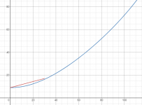
And this is an early simulation of Sandhorn + HF108 + DSA315-8 in the 74 liter enclosure with a passive radiator DSA315-PR.
This is not an ideal or the final, because it is based just on horizontal measurement of drivers and also there are visible resonance of cables inside enclosure, and reflections of the microphone stand in the measurements, but I'm posting this here just for an illustration how it could be...
This is not an ideal or the final, because it is based just on horizontal measurement of drivers and also there are visible resonance of cables inside enclosure, and reflections of the microphone stand in the measurements, but I'm posting this here just for an illustration how it could be...
Attachments
My initial thought was that it may be possible to model it without the driver internals (diaphragm, phase plug), which is not true as I see, so that somewhat loses its attraction.
It seems to me that all that is really needed is the distance from diaphragm to driver aperture and its radius. The volume of the chamber is likely just the diaphragm area by gap, and the gap is usually known.
If you are looking for tests that need no outside information, then that's going to be pretty hard. One thing that could be done is to drive the driver(2) with another source driver(1). Since you are looking for mostly the LF LP stuff, driver(1) does not have to be wide band width, nor does it need to be powerful. We did this kind of thing for cone speakers years ago. One can work out the equations and find the relationships, but, as I recall we still did not have enough to determine everything as a black box.
Just to be clear, you would also look at the blocked - at the aperture - Electrical impedance into Driver(2). I.E look both ways.
Last edited:
BTW, it's possible to simulate the first three axial duct modes as the source in the last Ath version (not documented). Simply put the following definition in the script:
Source.Contours = ::duct(w0, w1, w2)
Where w0, w1, w2 are the weights (amplitudes) of the 0th, 1st and 2nd mode.
Eg. duct(1.0, -0.5, 0.0)
It certainly works in the axisymmetric mode. Whether in the general 3D, I'm not sure at the moment.
Source.Contours = ::duct(w0, w1, w2)
Where w0, w1, w2 are the weights (amplitudes) of the 0th, 1st and 2nd mode.
Eg. duct(1.0, -0.5, 0.0)
It certainly works in the axisymmetric mode. Whether in the general 3D, I'm not sure at the moment.
Sorry, you've lost me. Are we still talking about measuring the exit wavefront shape?
That's what I thought you wanted originally, but then you said
"My initial thought was that it may be possible to model it without the driver internals (diaphragm, phase plug), which is not true as I see, so that somewhat loses its attraction."
The wavefront curvature is driver dependent and of course it will depend on specifics of the driver. The driver and the waveguide couple to each other and as such one cannot exclude the driver and get reliable and accurate data. It may be possible to ignore this couple, like using a rigid diaphragm to drive the waveguide, but this is not realistic and doing so will not yield accurate results.
A lot will depend on how much reflection there is in the waveguide (there is always some.) The lower the reflection the less important the boundary conditions of the driver are, but I doubt that they can ever be ignored in an accurate simulation.
I don’t think you’re likely to get better than a LE model of a compression driver in ABEC/Akabak unfortunately. There are some papers based on COMSOL for that purpose, and the model is quite far off without the use of a thermoviscous acoustics method for the narrow channels within the phase plug, and structure acoustics method to model the deformation of the diaphragm and surround.
Here's an example:
Compression Driver Simulation Including Air Damping in Phase Plug
What could possibly be done is to designate a nice, super detailed model of a particular compression driver in production and generate a very fine impedance mapping of the specific acoustic impedance across the exit. This could then be used as a data set for a surface driving impedance in ABEC, also known as a port boundary condition (I think, still learning - lot of this terminology!).
This, plus the graphical depictions of pressure wavefront shape might allow you to tailor the waveguide channel entry locations, lengths and curvature to get the spherical exit you want. It would restrict the resulting waveguide to one driver in principle, but if I'm honest that's kinda true for a lot of HF horns or waveguides but it doesn't stop people mixing it up.
Just found this as well:
https://uk.comsol.com/paper/download/292561/magalotti_presentation.pdf
Some good diagrams in there. But even more promisingly, it looks like the use of a boundary condition can compensate for thermoviscous losses without needing a full calculation based on Navier-Stokes:
Acoustic boundary layers as boundary conditions - ScienceDirect
I haven't read that paper yet, it's on 'the pile' but if someone with more spare time wants to dig in, it could be very useful for your purposes @mabat
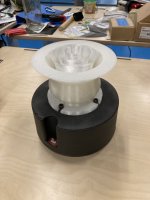
**Phase Plug Update**
So I have some good news and some bad news.
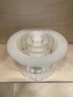
The good news is that the phase plug actually spreads the HF and improves loading.
Bad news is that it also introduces some peaks and dips. Especially on axis
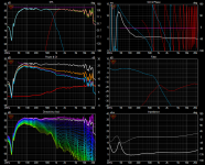
Just the Plug - 0, 15, 30 degrees

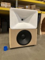
The plug mounted on a horn 0, 15, 30 degrees

On axis comparison of the phaseplug-axi-symmetirc horn vs rectangular horn

0 and 30 degree plots of the rectangular horn

The measurements vary in level as they are taken in different days and I don't really have a standartized jig for measuring yet. However I think they still hold up for comparison purposes.
So I have some good news and some bad news.
The good news is that the phase plug actually spreads the HF and improves loading.
Bad news is that it also introduces some peaks and dips. Especially on axis
Just the Plug - 0, 15, 30 degrees
The plug mounted on a horn 0, 15, 30 degrees
On axis comparison of the phaseplug-axi-symmetirc horn vs rectangular horn
0 and 30 degree plots of the rectangular horn
The measurements vary in level as they are taken in different days and I don't really have a standartized jig for measuring yet. However I think they still hold up for comparison purposes.
Attachments
What is going on with the impulse response of the red trace, which combination is that?On axis comparison of the phaseplug-axi-symmetirc horn vs rectangular horn
View attachment 996378
Background noise. There is a 3d printer in the background and the room is very reverberant
Blue trace is the Phase Plug Concentric Horn
Red trace is the Rectangular horn
An additional thing-
Only the first plot is a raw response of the driver and the plug.
In the other measurements, there is a basic, eq to flatten the "hump"
Blue trace is the Phase Plug Concentric Horn
Red trace is the Rectangular horn
An additional thing-
Only the first plot is a raw response of the driver and the plug.
In the other measurements, there is a basic, eq to flatten the "hump"
Last edited:
I'm talking about the number of reflections within 1ms in the red trace. That is not background noise, a printer or reverberation.Background noise. There is a 3d printer in the background and the room is very reverberant
Blue trace is the Phase Plug Concentric Horn
Red trace is the Rectangular horn
BTW nice job on the plug print
")
It explains why it looked strange, but it makes no sense to me to to look at an impulse response in metresOh, the impulse is measured in distance, in this case meters.
I hope that makes more sense
- Home
- Loudspeakers
- Multi-Way
- Acoustic Horn Design – The Easy Way (Ath4)