Jean Michel,
simulations cannot simply be assumed to be accurate, since almost any simulation is an approximation and they certainly cannot provide proof of an optimal or "best" solution. That would take maths.
I'm sure everyone here would be convinced if you could show mathematical proof that your horn profile has absolutely minimal diffraction.
Please don't feel offended, your intentions are good since you are trying to improve on things. But this is going to be a yes-no discussion, if we carry on with simulations and simple explanations without getting to the point: the maths behind this problem.
gedlee said:WIth enough computer power however the matrices could be analyzed with SVD,
Now finally something I understand! Nowadays unless your matrix is enormous, SVD takes very little time given a computer up to this decade standards. I do SVD almost daily, aka generalized inverses (not exactly the same but it is what you typically use SVD to compute).
john k... said:
It would seem that the OS wave guide is basically the right 1/2 of that picture with the profile set to a streamline that asymptotes to the correct exit angle (defining the profile hyperbola). So wouldn't the ideal diaphragm shape be that of an OS, i.e. the shape of a surface of constant velocity potential?
John
Absolutly correct. And it was exactly your picture (In Skudryks Foundations of Acoustics) that led me to the OS waveguide and the entire theory. I, like you, realized that this figure showed an exact solution of the problem in 3 dimensions and did not require the assumptions that limited Horn Theory. I later found that such a solution had already been performed by Freehaufer at MIT under the direction of Phillip Morse (not at all surprising!). He used a unique instrument called a "Differential Analyzer" which could solve differential equations mechanically. Today the numerical solutions have been done in Numerical Recipes and other texts. I used those solution techniques when I did the second paper identifying the HOMs and how they would be generated and propagate.
The geometry can be taken back to the origin, in which case the ideal source is a flat piston. An actual flat piston was used in the first OS waveguide experiments that proved that this geometry was indeed ideal for a flat piston. When the source is not flat other approachs must be use and the best source that I know of for that is in fact Chapter 6 of Audio Transducers.
JoshK said:
Now finally something I understand! Nowadays unless your matrix is enormous, SVD takes very little time given a computer up to this decade standards. I do SVD almost daily, aka generalized inverses (not exactly the same but it is what you typically use SVD to compute).
Absolutely, these days the SVD is easy, but getting the time to do it is the hard part. The point that I want to make is that I have been over this road, and while very interesting it doesn't lead to any change in what I am currently doing.
gedlee said:
Absolutely, these days the SVD is easy, but getting the time to do it is the hard part. The point that I want to make is that I have been over this road, and while very interesting it doesn't lead to any change in what I am currently doing.
Understood. Been there with my own work before. Ultimately, there are differences between practical significance and academic significance.
JoshK said:... there are differences between practical significance and academic significance.
Oh how true! I've been through all the academic work, now its time to make a practical success of that work.
gedlee said:
John
Absolutly correct. And it was exactly your picture (In Skudryks Foundations of Acoustics) that led me to the OS waveguide and the entire theory. I, like you, realized that this figure showed an exact solution of the problem in 3 dimensions and did not require the assumptions that limited Horn Theory. I later found that such a solution had already been performed by Freehaufer at MIT under the direction of Phillip Morse (not at all surprising!). He used a unique instrument called a "Differential Analyzer" which could solve differential equations mechanically. Today the numerical solutions have been done in Numerical Recipes and other texts. I used those solution techniques when I did the second paper identifying the HOMs and how they would be generated and propagate.
The geometry can be taken back to the origin, in which case the ideal source is a flat piston. An actual flat piston was used in the first OS waveguide experiments that proved that this geometry was indeed ideal for a flat piston. When the source is not flat other approachs must be use and the best source that I know of for that is in fact Chapter 6 of Audio Transducers.
Thanks for the conformation, Earl. One other thing, agreed that at the origin the potential surface is flat. However, The thing that has me wondering is that a surface of constant velocity potential is not (necessarily) a surface of constant velocity. This is certainly the case here since the potential surfaces are elliptical. Similarly, a surface of constant velocity would not be orthogonal to the stream lines, thus the velocity vector would not be perpendicular a surface of constant velocity. The point being that it would seem (nearly) impossible to actually construct a diaphragm which had pistonic motion and had the velocity vectors correctly aligned with the flow lines. Is this the origin of at least some of the HOMs? Also, are there other sources of HOMs, for example, arising at higher frequency due to relative comparison of wave length to WG dimensions, sort of like the HOM that are present in a constant area duct went the wave length is on the order of the duct cross sectional dimensions or smaller?
Hello a_tewinkel,
Simulations based on Boundary Elements Methods or Finite Elements Models, are math!
As they are based on solving the wave equation the accuracy is dependant on the geometrical definition ( size, shape of the elements , mesh....) and on the time increment between calculation steps.
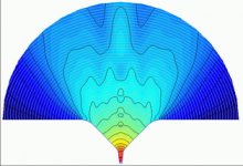
The map attached to my last message is obtained by a long duration simulation the most precise protocol, geometrical definition and time increments are more than optimal. Thus the result is for the most non contestable and will be approved by most audio scientists. BEM is a quasi standard of the industry when it comes to loudspeakers design, you cannot simply deny this fact.
You'll find here attached another map obtained with the exact same protocol than the map shown in my last message (surely you'll recognize that's it doesn't concern a Le Cléac'h horn...). Here you can see what are the bad effects of diffraction.
Best regards from Paris, France
Jean-Michel Le Cléac'h
Simulations based on Boundary Elements Methods or Finite Elements Models, are math!
As they are based on solving the wave equation the accuracy is dependant on the geometrical definition ( size, shape of the elements , mesh....) and on the time increment between calculation steps.
The map attached to my last message is obtained by a long duration simulation the most precise protocol, geometrical definition and time increments are more than optimal. Thus the result is for the most non contestable and will be approved by most audio scientists. BEM is a quasi standard of the industry when it comes to loudspeakers design, you cannot simply deny this fact.
You'll find here attached another map obtained with the exact same protocol than the map shown in my last message (surely you'll recognize that's it doesn't concern a Le Cléac'h horn...). Here you can see what are the bad effects of diffraction.
Best regards from Paris, France
Jean-Michel Le Cléac'h
a_tewinkel said:Jean Michel,
simulations cannot simply be assumed to be accurate, since almost any simulation is an approximation and they certainly cannot provide proof of an optimal or "best" solution. That would take maths.
I'm sure everyone here would be convinced if you could show mathematical proof that your horn profile has absolutely minimal diffraction.
Please don't feel offended, your intentions are good since you are trying to improve on things. But this is going to be a yes-no discussion, if we carry on with simulations and simple explanations without getting to the point: the maths behind this problem.
Attachments
john k... said:
Thanks for the conformation, Earl. One other thing, agreed that at the origin the potential surface is flat. However, The thing that has me wondering is that a surface of constant velocity potential is not (necessarily) a surface of constant velocity. This is certainly the case here since the potential surfaces are elliptical. Similarly, a surface of constant velocity would not be orthogonal to the stream lines, thus the velocity vector would not be perpendicular a surface of constant velocity. The point being that it would seem (nearly) impossible to actually construct a diaphragm which had pistonic motion and had the velocity vectors correctly aligned with the flow lines. Is this the origin of at least some of the HOMs? Also, are there other sources of HOMs, for example, arising at higher frequency due to relative comparison of wave length to WG dimensions, sort of like the HOM that are present in a constant area duct went the wave length is on the order of the duct cross sectional dimensions or smaller?
John
The wave equation that I use is in terms of pressure not velocity potential, hence the two variables are pressure and pressure gradient which is velocity. I suppose that it could be done in a velocity potential form (that is more common in CFD than acoustics), but that's not the way I did it nor have I seen that done. The fact that the pressure gradient at the origin is a function of the distance from the axis is described in my past writings which shows how a uniform velocity will still generate HOMs. This function also changes with frequency and so it is highly unlikely that BOTH the velocity contour and the change in frequency could be achieved simultaneously. However, I do show how one could surpress any desired mode by velocity shaping, and one of my patents describes how to do this.
The nonorthogonal nature of the velocity to the pressure is the reason for the HOMs that are generated within the device. And all devices where the wavefront shape is changing will have these. The HOMs that are created by a mismatch of the source to the duct are another issue. Those HOMs are created by the boundary conditions at the throat.
The HOM do have a cut-in phenomina exacty like waves in a duct and they exist, just like in the duct, depending on how the source is aligned with the duct. A duct fed with a flat plane wave will not have HOMs even if it is possible for them to exist. Everything depends on how the source fits onto the duct.
This is why I don't believe Jean-Michels simulations. The throat does not look right to me and its very easy to get that wrong. Even easier if thats what you want to do. Comparing a single frequency from one device to another is also meaningless as other frequencies may be completely different.
Below some cutoff the HOM are "evanescent" in any duct straight or flared. They exist and propagate but with a complex wavenumber which makes them attenuate with distance exponentially. BUT in a short device these waves COULD make it to the mouth and still be part of the radiation. Its a complex problem.
The HOM probably do in fact travel at different speeds just like the unflared duct (everything else is similar) but it would be a complex mathematical problem to calculate that speed. Maybe not so complex, just not something that I have done.
The HOM probably do in fact travel at different speeds just like the unflared duct (everything else is similar) but it would be a complex mathematical problem to calculate that speed. Maybe not so complex, just not something that I have done.
Hello Earl,
What you wrote is very unfair and could be even considered as insulting. The truth is that the same care has been put in every simulation and even you advice was required to help in designing several aspects of the OS waveguide.
We presented the results at many different frequencies for both horn and waveguide.
An important feature that seems important in understanding the behavior of a horn or a waveguide is the reflection coefficient curve. For the Le Cleac'h horns that have been measured the smoothness of the reflection coefficient curve and the low value it presents compared to conical horns and waveguides is perfectly reflected in the group delay curve derived from the pulse analysis and also in the absence of parasitic artefacts in the electric impedance curve.
Until now there is no discrepancy between the simulations performed on the Le Cléac'h horn, the hypothesis at the basis of its design and the measurements performed. A batch of new measurements (open door) should arrive and we'll publish the results on the DIYaudio forum (on the "other" thread naturally).
Best regards from Paris,
Jean-Michel Le Cléac'h
gedlee said:
This is why I don't believe Jean-Michels simulations. The throat does not look right to me and its very easy to get that wrong. Even easier if thats what you want to do. Comparing a single frequency from one device to another is also meaningless as other frequencies may be completely different.
Jmmlc said:Hello Earl,
The truth is that the same care has been put in every simulation and even you advice was required to help in designing several aspects of the OS waveguide.
Best regards from Paris,
Jean-Michel Le Cléac'h
I said when I first saw those that I did not think that the throat looked right and asked to see it it more detail so that I could check it. This request was ignored. That is NOT taking "the same care" as you claim. That is ignoring a direct complaint about this care. I never checked what was done - thats not care, thats negelect.
Earl,
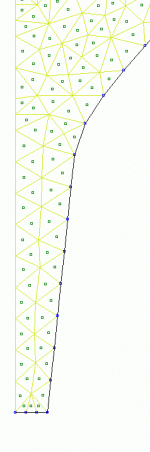
Checking back, I see that you did post a request. Sorry for not recognizing it. Here is a close-up of half the throat of the waveguide used in the simulation. Element length is no more than 1/6th wavelength at 8kHz. Blue rectangles are nodes, green rectangles are field points.
From what you write, it may be necessary to use a denser boundary mesh to get things right.
Bjørn
Attachments
Kolbrek said:Earl,
Checking back, I see that you did post a request. Sorry for not recognizing it. Here is a close-up of half the throat of the waveguide used in the simulation. Element length is no more than 1/6th wavelength at 8kHz. Blue rectangles are nodes, green rectangles are field points.
From what you write, it may be necessary to use a denser boundary mesh to get things right.
Bjørn
Bjorn
First the throat seems way too long. I don't know the actual length of the throat in the DE250, you would have to get that data from B&C. I also don't have the actual data point values to check either.
If these sims are going to be used at "attack" a design then you have to be sure that they are correct. Jean-Michel is unfairly using the results IMO by showing only what he wants us to see. If he is getting these from you then it is only fair that everyone be able to see all the results that are available and concur with the process. Can you do far field polar amps? These are only near field and only single frequency, not really very enlightening at all. If you have trouble plotting polar maps then I would do that for you as I have this capability. I would just need far-field results of SPL versus angle and frequency.
And, yes, that is a very coarse mesh for a high frequency. One should usually have about six elements per wavelength. With what you have shown the HF limit of accuracy would only be 6-8 kHz. If the density is too coarse then you know that this will generate aberations that are not accurate and these aberation will differ from device to device, none of which is correct.
I also question the validity of going all the way back into the throat of the device since this is part of the driver NOT part of the waveguide. The waveguide cannot correct for the drivers deficiencies and different drivers will act differently. I suggest that the two devices be compared driver independent, i.e. just the waveguide/horn portion, without the driver. If this is a model of actual devices then why not just use actual devices? We have those devices and the driver, why not just compare them directly? Why the need for a model? Models are used when the reality is not available, but in this case we have reality.
I would be more than willing to do the measurements if I could get one of Jean-Michels horns. Someone could be here to oversea the tests, thats fine with me. But I don't think that anyone is questioning my ability to perform the tests, I've done lots and lots of them over the last decade. If Jean-Michel is so intent on a competition then let's have one, but lets make it fair, not this one-sided stuff that we have been seeing. That is most unprofessional.
gedlee said:If these sims are going to be used at "attack" a design then you have to be sure that they are correct. Jean-Michel is unfairly using the results IMO by showing only what he wants us to see. If he is getting these from you then it is only fair that everyone be able to see all the results that are available and concur with the process.
I'm not happy with the direction this discussion has taken either, to the point of regretting sharing these simulations at all.
 I don't want to be part of this discussion of OS waveguide vs. Le Cléac'h horn. I did some simulations out of curiosity, not to make ammunition for an "attack".
 Surely I could generate lots of data for a discussion like this, but I want to stay out of it. I don't have time for it.
Can you do far field polar amps? These are only near field and only single frequency, not really very enlightening at all. If you have trouble plotting polar maps then I would do that for you as I have this capability. I would just need far-field results of SPL versus angle and frequency.
I can't do it at the moment, but I plan to add this capability to my SW. I attach the far field field (3m) point data, for a fixed throat velocity, from the simulation I did in the "Beyond the Ariel" thread. It's a text file format, zipped because of size constraints. It should be fairly easy to interpret. It's the same boundary profile that I used for the field plots, exept that it is twice as dense, since the maximum frequency is 15kHz.
And, yes, that is a very coarse mesh for a high frequency. One should usually have about six elements per wavelength. With what you have shown the HF limit of accuracy would only be 6-8 kHz.
That's just what I said, 6 elements per wavelength (element size no greater than 1/6th WL at 8kHz), and 8kHz is the highest frequency used in the field plots. One will of course try to keep the size down, as computation time increases with the square of the number of elements.
Bjørn
Attachments
goskers said:Now we are talking!!
I would love to see a head to head with the LeCleac'h horn and a GedLee WG.
Who's taking bets as I'd like to make a wager
but how does one measure, much less quantify, the feeling in the spine of the experience of great music?
that emotional involvement that makes one quit analyzing, and get lost in the enjoyment of music...
counting the number of hairs that stand up on the back of the neck?
- Home
- Loudspeakers
- Multi-Way
- Geddes on Waveguides