What do you think makes NOS sound different?

[Ken Newton]

You can make DAC to "color" the sound if that's what one desires but it has so much more limitations in that aspect than equalizer, speakers and room acoustics. However, I'm not trying to stop you from doing what you enjoy doing.

Good. That then ends questions of why I’m not not simply accepting when someone else tells me that a given component is perfect, because the available specs. dictate that it must be.

False assertion? There are level matched double blind listening tests reporting audibly indistinguishable between high-end DAC and cheap mass produced receiver DAC. I see that you left out the word "audibly" which I used. It is the primary aspect when dealing with audio gear, no?

Yes, false, for those of us who hear a seemingly inexplicable difference between OS and NOS, or have you not been following the thread?

You asked me something out of curiosity and I answered. I asked you something out of curiosity as well…Which method do you use for ensuring that, computer, your own ears or something else?

Okay, I’ll play along, just a bit. Room modes and reflections make it very unlikely that the sound at my listening position is anywhere near flat. I don’t apply any room correcting DSP or EQ. I largely utilize the speaker positioning principles of Roy Allison, and, especially, Stig Carlsson. Which means that my speakers are located against the front wall of the listening room, my listening position is relatively close to the speakers, which are toed in so that their directivity crosses just in front of my head. This has given me the most subjectively natural tonality I’ve experienced from my speakers. That should suffice as an answer.

 

[Hans Polak]

I think 1/2 LSB peak-peak of uniformly distributed differential dither can take care of the noise modulation, see the bottom of page 7 and top of page 8 of the attachment.

That was what I planned today to do in more detail.
I already tried with 0.1LSB rms HF noise mixed with the signal and that seemed to go fine.

Hans

 

[Hans Polak]

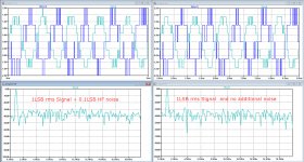
Here the results of some experiments, but first a resume:

1) Tri Dither with an 0.4 LSB RMS value was added in opposite phase two differential Dacs, and after differential D/A conversion cancelled as common mode in a diff amp.
2) With a signal of enough amplitude added to the opposite dither signals, and after D/A conversion processed as differential signals, a gain in S/N of ca 10dB was achieved compared to a Dac processing signal and dither in the usual way.
3) However for a DC signal or a very low level signal, output noise dropped by 80dB because of this common mode noise cancellation scheme, resulting in noise modulation.
4) To prevent this from happening, a new uncorrelated source was added directly to the Signal, effectively leaving the Dac's as differential noise just like the signal itself.
5) for this additional noise a 0.1LSB rms noise source was used, 12 dB below the dither noise and bandlimited at around 10Khz, an area where our auditory system is less sensitive, just as an idea without mathematical backup.

In the images below, the time domain signal of one Dac and the output signal are shown, where in the latter the CM component was removed.
The spectrum below this time domain part shows the spectrum of the output signal.

In the first image a 1LSB rms 1Khz signal was used.
Left side shows the result with the added 0.1LSB rms and the right side shows the same for having added no additional noise.
Adding the 0.1LSB rms noise seems to have no visible effect on the level of the noise spectra between the two output signals..

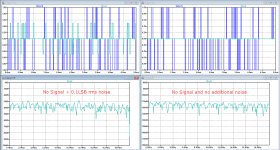
Second image shows the same, but now without the 1Khz signal.
At the left, where the 0.1LSB noise was added, the output spectrum's noise level is still identical to the first image with the 1Khz signal.
However the right side with no additional 0.1LSB rms noise is showing a spectrum that went from ca -40dB to -120dB, note the the different scales.

So adding just this little bit of noise to the signal does not result in a visible noise level increase at the output, but it seems to completely prevent noise modulation.

Hans
.

 

[Ken Newton]

...So adding just this little bit of noise to the signal does not result in a visible noise level increase at the output, but it seems to completely prevent noise modulation.

Hans
.

Real good work, Hans. Marcel is a wizard at mathematical modeling, but your translation of his models in to a circuit simulation really helps in seeing what the math predicts.

So, if I correctly understand your simulation, 0.4 LSB of rectangular dither is summed to appear as common-mode noise at the outputs of the differential DACs, while 0.1 LSB of an independent rectangular dither is summed to appear as a residual (is not subsequently subtracted) difference-mode noise at the outputs of the differential DACs?

 

[Hans Polak]

Yes Ken, completely correct, with the small addition that in this example the 0.1LSB rms noise was band filtered around 10Khz, but that may not be necessary at all.

Hans

 

[MarcelvdG]

Theoretically it should be 0.5 LSB peak-peak uniformly distributed, so that's about 0.1443375673 LSB RMS, that level should suffice both for the common- and for the differential-mode dither. You can use an integer multiple of that (an even multiple anyway) for the common-mode dither when you want to randomize errors due to DNL.

Anyway, nice to see that theory and simulations (qualitatively) match!

 

[Evenharmonics]

Good. That then ends questions of why I’m not not simply accepting when someone else tells me that a given component is perfect, because the available specs. dictate that it must be.

When audibility threshold is known by listening test correlated with measurements, you can figure out what's below or above audible range by looking at the measurements of DAC. Distortion / jitter below audible range has been reached decades ago for cheap mass produced DACs.

Yes, false, for those of us who hear a seemingly inexplicable difference between OS and NOS, or have you not been following the thread?

You mean perceive inexplicable difference? Because whether it's actually heard or not will be confirmed after objective analysis.

Okay, I’ll play along, just a bit. Room modes and reflections make it very unlikely that the sound at my listening position is anywhere near flat. I don’t apply any room correcting DSP or EQ. I largely utilize the speaker positioning principles of Roy Allison, and, especially, Stig Carlsson. Which means that my speakers are located against the front wall of the listening room, my listening position is relatively close to the speakers, which are toed in so that their directivity crosses just in front of my head. This has given me the most subjectively natural tonality I’ve experienced from my speakers. That should suffice as an answer.

So you just use your ears. That's what I thought. By the way, no speakers in the room (typical consumer's room) is ever flat in frequency response at the listening spot, ever!
If you have time, try this for your listening spot.

 

[Hans Polak]

Theoretically it should be 0.5 LSB peak-peak uniformly distributed, so that's about 0.1443375673 LSB RMS, that level should suffice both for the common- and for the differential-mode dither. You can use an integer multiple of that (an even multiple anyway) for the common-mode dither when you want to randomize errors due to DNL.

Anyway, nice to see that theory and simulations (qualitatively) match!

Hi Marcel,
A few things.

1) I’m using LTSpice’s white noise generator, of which I assume that it is Gaussian distributed instead of rectangular, that’s why I’m using rms values instead of peak-peak values.

2) Quantisation noise has an rms value of 0,288 LSB rms.
Tri dither is supposed to be sqrt(2) higher at 0.4 LSB rms to get noise decorrelated from the signal, true ?
So I don’t get your 0.144 LSB rms for the common mode dither.
In this very case the level of the common mode dither plays hardly a role as long as it is =>0.4 LSB rms.
When using 1.6LSB rms or four times as much for the common mode dither, the noise level at the output after common mode removal stays the same.

3) The differential mode noise should stay well below the quantisation noise of 0.288 LSB rms, so yes, I agree that 0.144 could have been used instead of 0.1 LSB rms, output noise would then increase by 1dB instead of the 0.5dB in my case, both are o.k.

Am I making an error somewhere ?

Hans

 

[MarcelvdG]

Depending on how you arrange the rounding and what the DC value of the dither is, you can get the DACs to take steps in turn, so that they together behave as an N + 1 bit DAC. Hence you can use half the dither that you would need with a single DAC. See the appendix of my latest document for an example.

There is no point in using triangular noise for the common-mode dither, because you can't avoid noise modulation with (only) common-mode dither anyway. That's why I suggested rectangular common-mode dither. You can then use another rectangularly distributed noise signal for differential dither to get rid of the noise modulation.

According to pages 104 and 105 of http://www.ieca-inc.com/images/LTSPICE_Manual.pdf , rand(x) and random(x) generate random numbers between 0 and 1 and white(x) between -0.5 and 0.5, but it doesn't say with what distribution. I would guess uniform because computer random number generators are usually uniform by default, but that's just a guess. If it were Gaussian it would have to be truncated Gaussian to guarantee that the value remains between the limits.

According to LTspice: Worst-Case Circuit Analysis with Minimal Simulations Runs | Analog Devices there are also functions gauss(x) and flat(x) with Gaussian and uniform distributions, but I don't know if you can use them with an arbitrary voltage source.

There are no correct dither levels with Gaussian dither, it just gradually gets better (and more noisy) as the level increases. A rule of thumb is that it works reasonably well when the dither noise power is at least 1.5 times the noise power of triangular dither, so 3 times the usual quantization error power.

 

[Ken Newton]

When audibility threshold is known by listening test correlated with measurements, you can figure out what's below or above audible range by looking at the measurements of DAC. Distortion / jitter below audible range has been reached decades ago for cheap mass produced DACs.


You mean perceive inexplicable difference? Because whether it's actually heard or not will be confirmed after objective analysis.


So you just use your ears. That's what I thought. By the way, no speakers in the room (typical consumer's room) is ever flat in frequency response at the listening spot, ever!
If you have time, try this for your listening spot.

I'm finished with the discussion. You had the last word above.

 

[roderickvd]

According to pages 104 and 105 of http://www.ieca-inc.com/images/LTSPICE_Manual.pdf , rand(x) and random(x) generate random numbers between 0 and 1 and white(x) between -0.5 and 0.5, but it doesn't say with what distribution. I would guess uniform because computer random number generators are usually uniform by default, but that's just a guess. If it were Gaussian it would have to be truncated Gaussian to guarantee that the value remains between the limits.

"White" sounds like it's Gaussian.

When Gaussian functions are used as the pdf of a normal distribution, they can be limited and do not need to be truncated.

There are no correct dither levels with Gaussian dither, it just gradually gets better (and more noisy) as the level increases. A rule of thumb is that it works reasonably well when the dither noise power is at least 1.5 times the noise power of triangular dither, so 3 times the usual quantization error power.

According to this paper Gaussian dither should be 1/2 LSB *RMS*, not peak-to-peak, to linearise the output. So that's a normal distribution with μ=0 and σ=0.5.

 

[MarcelvdG]

White just means no autocorrelation, the PDF can be anything. How do you keep the extremes of a Gaussian distribution finite without truncation?

As the usual approximation for the RMS quantization error is 1/sqrt(12) LSB, 1/2 LSB RMS is sqrt(3) times as much, so 3 times the power, precisely the rule of thumb that I quoted.

 

[roderickvd]

White just means no autocorrelation, the PDF can be anything.

Yes I'm sorry, you're quite right.

How do you keep the extremes of a Gaussian distribution finite without truncation?

When we're talking about Gaussian functions as a pdf for normal distributions, is the maximum value not determined by 1/(sqrt(2π)*σ), so for σ=0,5 this is approximates 0,8?

As the usual approximation for the RMS quantization error is 1/sqrt(12) LSB, 1/2 LSB RMS is sqrt(3) times as much, so 3 times the power, precisely the rule of thumb that I quoted.

Sorry if my statistics are getting rusty, trying to contribute here and not at all question your knowledge!

 

[Hans Polak]

There is no point in using triangular noise for the common-mode dither, because you can't avoid noise modulation with (only) common-mode dither anyway. That's why I suggested rectangular common-mode dither.

Each Dac is on its own before it’s output is processed by a diff amp.
So why deviate from the rule to use tri dither of 0.4 LSB rms to prevent noise modulation, and why use rectangular noise of only 0.144 LSB rms when this results in modulated noise ?
I don’t see how the diff amp that can repair that.

You can then use another rectangularly distributed noise signal for differential dither to get rid of the noise modulation.

That is exactly what I did, so here we are in agreement concerning sort and level of the differential noise.

According to pages 104 and 105 of 404 Not Found , rand(x) and random(x) generate random numbers between 0 and 1 and white(x) between -0.5 and 0.5, but it doesn't say with what distribution. I would guess uniform because computer random number generators are usually uniform by default

When analysing White(x) over a longer time, variance should be 1/12, but it is 27% less with 0.061, so its not uniform.

There are no correct dither levels with Gaussian dither, it just gradually gets better (and more noisy) as the level increases. A rule of thumb is that it works reasonably well when the dither noise power is at least 1.5 times the noise power of triangular dither, so 3 times the usual quantization error power.

O.k thx, good to know.

 

[MarcelvdG]

If it were Gaussian with 0.5 as three-sigma value (assuming tails beyond three sigma are cut off), the variance would be 1/36 = 0.02777... Apparently white() is neither uniform nor Gaussian. Not exactly triangular either.

 

[MarcelvdG]

When we're talking about Gaussian functions as a pdf for normal distributions, is the maximum value not determined by 1/(sqrt(2π)*σ), so for σ=0,5 this is approximates 0,8?

I shouldn't have used the word truncation. I meant cutting off the tails, not rounding towards zero.

With a Gaussian distribution, any value has a nonzero probability density, so you have to cut off tails to keep it finite at all times. Or at least that's how I see it.

 

[scott wurcer]

Hi Marcel,
A few things.

1) I’m using LTSpice’s white noise generator, of which I assume that it is Gaussian distributed instead of rectangular, that’s why I’m using rms values instead of peak-peak values.

Hans I've said this before, LTSpice is a nice tool and service to the DIY community but it is not a general purpose research tool. The fully vetted IEEE math library is available for free in any number of tools. You have available more statistical functions (random number generators, etc.) than you could ever use all fully described and used by almost all scientific organizations, CERN, LIGO, etc.

Simple random data
rand(d0, d1, …, dn) Random values in a given shape.
randn(d0, d1, …, dn) Return a sample (or samples) from the “standard normal” distribution.
randint(low[, high, size, dtype]) Return random integers from low (inclusive) to high (exclusive).
random_integers(low[, high, size]) Random integers of type np.int between low and high, inclusive.
random_sample([size]) Return random floats in the half-open interval [0.0, 1.0).
random([size]) Return random floats in the half-open interval [0.0, 1.0).
ranf([size]) Return random floats in the half-open interval [0.0, 1.0).
sample([size]) Return random floats in the half-open interval [0.0, 1.0).
choice(a[, size, replace, p]) Generates a random sample from a given 1-D array
bytes(length) Return random bytes.

Permutations

shuffle(x) Modify a sequence in-place by shuffling its contents.
permutation(x) Randomly permute a sequence, or return a permuted range.
Distributions
beta(a, b[, size]) Draw samples from a Beta distribution.
binomial(n, p[, size]) Draw samples from a binomial distribution.
chisquare(df[, size]) Draw samples from a chi-square distribution.
dirichlet(alpha[, size]) Draw samples from the Dirichlet distribution.
exponential([scale, size]) Draw samples from an exponential distribution.
f(dfnum, dfden[, size]) Draw samples from an F distribution.
gamma(shape[, scale, size]) Draw samples from a Gamma distribution.
geometric(p[, size]) Draw samples from the geometric distribution.
gumbel([loc, scale, size]) Draw samples from a Gumbel distribution.
hypergeometric(ngood, nbad, nsample[, size]) Draw samples from a Hypergeometric distribution.
laplace([loc, scale, size]) Draw samples from the Laplace or double exponential distribution with specified location (or mean) and scale (decay).
logistic([loc, scale, size]) Draw samples from a logistic distribution.
lognormal([mean, sigma, size]) Draw samples from a log-normal distribution.
logseries(p[, size]) Draw samples from a logarithmic series distribution.
multinomial(n, pvals[, size]) Draw samples from a multinomial distribution.
multivariate_normal(mean, cov[, size, …) Draw random samples from a multivariate normal distribution.
negative_binomial(n, p[, size]) Draw samples from a negative binomial distribution.
noncentral_chisquare(df, nonc[, size]) Draw samples from a noncentral chi-square distribution.
noncentral_f(dfnum, dfden, nonc[, size]) Draw samples from the noncentral F distribution.
normal([loc, scale, size]) Draw random samples from a normal (Gaussian) distribution.
pareto(a[, size]) Draw samples from a Pareto II or Lomax distribution with specified shape.
poisson([lam, size]) Draw samples from a Poisson distribution.
power(a[, size]) Draws samples in [0, 1] from a power distribution with positive exponent a - 1.
rayleigh([scale, size]) Draw samples from a Rayleigh distribution.
standard_cauchy([size]) Draw samples from a standard Cauchy distribution with mode = 0.
standard_exponential([size]) Draw samples from the standard exponential distribution.
standard_gamma(shape[, size]) Draw samples from a standard Gamma distribution.
standard_normal([size]) Draw samples from a standard Normal distribution (mean=0, stdev=1).
standard_t(df[, size]) Draw samples from a standard Student’s t distribution with df degrees of freedom.
triangular(left, mode, right[, size]) Draw samples from the triangular distribution over the interval [left, right].
uniform([low, high, size]) Draw samples from a uniform distribution.
vonmises(mu, kappa[, size]) Draw samples from a von Mises distribution.
wald(mean, scale[, size]) Draw samples from a Wald, or inverse Gaussian, distribution.
weibull(a[, size]) Draw samples from a Weibull distribution.
zipf(a[, size]) Draw samples from a Zipf distribution.

 

[MarcelvdG]

Each Dac is on its own before it’s output is processed by a diff amp.
So why deviate from the rule to use tri dither of 0.4 LSB rms to prevent noise modulation, and why use rectangular noise of only 0.144 LSB rms when this results in modulated noise ?
I don’t see how the diff amp that can repair that.

You have demonstrated that unmodulated noise from both DACs doesn't guarantee that the difference is unmodulated - as the noise is not independent, noise from one DAC can cancel noise from the other DAC. In my scheme they complement rather than cancel each other: in each 1/2 LSB interval, one produces noise while the other doesn't. The total noise is periodic as a function of the input signal with a period of 1/2 LSB, which is solved by randomizing over 1/2 LSB with the differential dither.

 

[scott wurcer]

I shouldn't have used the word truncation. I meant cutting off the tails, not rounding towards zero.

With a Gaussian distribution, any value has a nonzero probability density, so you have to cut off tails to keep it finite at all times. Or at least that's how I see it.

Not quite that simple, https://www.doc.ic.ac.uk/~wl/papers/07/csur07dt.pdf

Bottom line these days it's pretty easy to get 9 sigma (the Box-Muller method does this at 64 bit integer resolution). This is not a factor in any audio application.

 

[roderickvd]

I shouldn't have used the word truncation. I meant cutting off the tails, not rounding towards zero.

Yes, that's also how I understood it. I'm curious though why you would want to do that? While I haven't done the math, by breaking its continuinity I hypothesize that it introduces non-linearity or, put differently, reduces the linearizing effect of the dither.

As you have also stated, it's known that Gaussian dither has greater noise power compared to RPDF or TPDF, which to me seems reflected not only by the larger surface under the curve but also "overflowing" into 2 LSB territory rather than the 1 LSB of RPDF or TPDF.

With a Gaussian distribution, any value has a nonzero probability density, so you have to cut off tails to keep it finite at all times. Or at least that's how I see it.

I'm not sure I'm following. Maybe we're talking about different things - a Gaussian distribution versus a normal distribution with a Gaussian pdf?

Certainly for a normal distribution with μ=0 and σ=0.5 the probability of, let's exaggarate, an x-value of 10 is zero.
Even then, why would it matter to keep it finite (as long as the probability decreases as the values move away from zero?)

Which makes me wonder about the merits of Gaussian PDF at all. If I recall correctly, Wannamaker wrote that for every "n" of RPDF dither, an "n" order of system output is rendered independent, which is the mechanism by which linearization occurs. Again IIRC, he wrote that with TPDF being 2RPDF, greater n-levels may be worthwhile in video applications but not in audio applications.

Now thinking that GPDF is RPDF with n=infinite by merits of the central limit theorem, and assuming that n>2 is not worthwhile for audio applications, where does that leave us? I have found some statements that since GPDF is akin to the white noise of analog sources, as well as having a greater noise power, it may sound more "analog". But I'd be fooling myself if I thought I could actually discern between GPDF and TPDF in 24-bit. Probably even in 16-bit it'd be a stretch.