I spent way to long the last few days trying to write a function to tracing out the different mode lines from the slanted side study I posted previously. Tried simple linear difference estimator from previous two or three points, also tried to estimate curvature with a simple diff of diffs, but it seems the data is too noisy for those simple estimates to be stable.
Best so far is a simple least-squares line of best fit through the previous three points, results shown below. I may at some point knuckle down and try a quadratic least squares on the last 4-5 points, but for now I'm moving on. (I asked about a globally optimal algorithm on Stack Overflow but the question was immediately canned as unclear.)
There also be some lines missing bc I have not bothered to implement a final loop to check all data has been accounted for.
OMG Paul,I spent way to long the last few days trying to write a function to tracing out the different mode lines from the slanted side study I posted previously. Tried simple linear difference estimator from previous two or three points, also tried to estimate curvature with a simple diff of diffs, but it seems the data is too noisy for those simple estimates to be stable.
Best so far is a simple least-squares line of best fit through the previous three points, results shown below. I may at some point knuckle down and try a quadratic least squares on the last 4-5 points, but for now I'm moving on. (I asked about a globally optimal algorithm on Stack Overflow but the question was immediately canned as unclear.)
There also be some lines missing bc I have not bothered to implement a final loop to check all data has been accounted for.
View attachment 1132785
Sorry I didn't mean for that to happen! If you really want to, there is the brute force method....that is....looking at the mode shapes and attaching similar mode shapes to the same line. Not sure it's worth the effort however. I did it for the case below, but I had fewer modes and fewer steps. It could work if you really want to do it.
Eric
Not your fault, Eric, I was interested to do it!OMG Paul,
Sorry I didn't mean for that to happen! If you really want to, there is the brute force method....that is....looking at the mode shapes and attaching similar mode shapes to the same line. Not sure it's worth the effort however. I did it for the case below, but I had fewer modes and fewer steps. It could work if you really want to do it.
Eric
View attachment 1132804
But its not so easy (and still less easy if I were to have pretensions of statistical rigour). Still, the graph above is interesting and does show many instances where the modes diverge, even though its is biased toward continuing a straight line (strictly linear regression) rather than recognising the presence of curvature.
If I understand your suggestion, I'm afraid that writing software to recognise similarity of mode shapes is an even more difficult problem.
Hello PaulNot your fault, Eric, I was interested to do it!
But its not so easy (and still less easy if I were to have pretensions of statistical rigour). Still, the graph above is interesting and does show many instances where the modes diverge, even though its is biased toward continuing a straight line (strictly linear regression) rather than recognising the presence of curvature.
If I understand your suggestion, I'm afraid that writing software to recognise similarity of mode shapes is an even more difficult problem.
I like the way you are searching. Close to my "classical" methods.
About the least square, I have to read more carefully to what you want to do to see if I can help (not possible to concentrate enough for now).
About the mode recognition, if you can get the mode shapes from Elmer under a numpy array, I have a code doing that( works for simply supported and clamped conditions on a rectangular plate, not tested under other conditions : slant for exemple) . See attached file. I tried to add comment you can use it. Tell me for additional comments.
Christian
Attachments
If I understand your suggestion, I'm afraid that writing software to recognise similarity of mode shapes is an even more difficult problem.
Haha, nope, I meant even more brute force than that...actually looking with your own eyes is what I meant!
I understand of course that's not a practical "general" solution. But I'm just really curious whether or not there are more line crossings than your graph suggests.
It's interesting to look at your graph by turning the screen at an angle, effectively squeezing the graph from left to right and giving you a different perspective. Try it if you have not already.
I think you could pick just a few modes that come close to crossing, and examine the mode shapes associated with them at a few points (say at side slant values of 0, 0.1, 0.2, 0.3 .......0.9, 1.0) you might be able to tell for certain whether or not the lines actually cross or not.
Three modes that looks interesting are the one that (at slant=0) is at nearly exactly 100 Hz, and the two lines/modes just below it. If I ignore your colors, my eyes "want" them to cross two or maybe three times (at around 0.15, 0.35, and maybe 0.75). If you inspected the modes shapes of those three modes at just a few points along the "slant" axis, you could probably tell if the lines cross or not.
If nothing else it would help to verify whether or not your tracing algorithm is working.
Eric
Christian,About the mode recognition, if you can get the mode shapes from Elmer under a numpy array, I have a code doing that( works for simply supported and clamped conditions on a rectangular plate, not tested under other conditions : slant for exemple) . See attached file. I tried to add comment you can use it. Tell me for additional comments.
That's amazing. Can you describe the strategy (just the basic idea, not every detail)?
Eric
Hi EricChristian,
That's amazing. Can you describe the strategy (just the basic idea, not every detail)?
Eric
Yes for sure.
The plate is divide is divided in each direction. The displacement is computed on each point of the picture below.
Different kind of simulation are possible : with a driving point in frequency, over the time (transient). The current script computes the modes. Python with its library Scipy offers the possibility to get the eigenfrequencies AND the corresponding mode shapes, as you very often show from Lisa
The "mode detection algorithm" search for the maximum (the red dot), being positive or negative in those mode shapes which are 2D matrix corresponding to the plate geometry. Probably there are several points with the same values or about, it doesn't matter.
From the coordinates of this point, the algorithm makes a section in the x direction (m of the modes), an other in the y (n of the modes).
The cross section is the deviation of each points along the chosen direction.
The trick is in the idea to detect how many times the sign (positive, negative) of the deviation changes along the section and then add one.

The code I found from Stackoverflow help me a lot to write it in few Python lines.
With that, it is possible to retro-annotate the figures with the m,n, compute from existing formulas the expected mode frequency and check the accuracy of the method or more simply if the values are plausible.
The power of Python! Think to it! Joke aside, Python is really an affordable language with library oriented to sciences and engineering. There are many tuto, free books. Paul shown us the possibilities of pre or post processing with Elmer. The step after Excel!
Christian
So awesome! Neat.Hi Eric
Yes for sure.
PaulI think you could pick just a few modes that come close to crossing, and examine the mode shapes associated with them at a few points (say at side slant values of 0, 0.1, 0.2, 0.3 .......0.9, 1.0) you might be able to tell for certain whether or not the lines actually cross or not.
Three modes that looks interesting are the one that (at slant=0) is at nearly exactly 100 Hz, and the two lines/modes just below it. If I ignore your colors, my eyes "want" them to cross two or maybe three times (at around 0.15, 0.35, and maybe 0.75). If you inspected the modes shapes of those three modes at just a few points along the "slant" axis, you could probably tell if the lines cross or not.
I took a stab at this myself and realized it was folly to try. Once I got to "slant=0.4" many mode shapes were unrecognizable. What the heck is this for example?
Up to slant=0.2 all the modes where easy to recognize, at least up to 200 Hz (where I stopped). Interestingly, the modes I originally thought were crossing at about "slant=0.15" were the 2,4 and 3,1 modes. But it appears now to me that they do not cross after all, as you said.
Eric
Paul, Christian,
I would be very interested to compare the results of all our models for a particular simple case. I'm especially interested to see how Elmer compares to LISA, since Elmer uses Mindlin elements while LISA does not. And then, which is Christians FDM closer to? I expect to the see models be pretty close at low frequency but diverge more and more as frequency increases, as a result of shear.
Would you guys run your models for me with the conditions below and let me know what you get?
Below are the LISA results for the following conditions:
Size: 1.2 m x .35 m x .004 m
E= 8 GPa
poissons ratio = 0.2
supports: simple all edges.
Hello EricPaul, Christian,
I would be very interested to compare the results of all our models for a particular simple case. I'm especially interested to see how Elmer compares to LISA, since Elmer uses Mindlin elements while LISA does not. And then, which is Christians FDM closer to? I expect to the see models be pretty close at low frequency but diverge more and more as frequency increases, as a result of shear.
Would you guys run your models for me with the conditions below and let me know what you get?
Below are the LISA results for the following conditions:
Size: 1.2 m x .35 m x .004 m
E= 8 GPa
poissons ratio = 0.2
supports: simple all edges.
Which density ?
Christian
SorryHello Eric
Which density ?
Christian
500 kg/m3
Hi EricPaul
I took a stab at this myself and realized it was folly to try. Once I got to "slant=0.4" many mode shapes were unrecognizable. What the heck is this for example?
View attachment 1133084
Up to slant=0.2 all the modes where easy to recognize, at least up to 200 Hz (where I stopped). Interestingly, the modes I originally thought were crossing at about "slant=0.15" were the 2,4 and 3,1 modes. But it appears now to me that they do not cross after all, as you said.
Eric
That case I would say is fairly uncontroversial, because you can see a gap maintained over many samples, and because the curves anticipate the crossing point and flatten out.
This phenomenon seems to have a name, originally from quantum physics, called ‘level repulsion’. It happens in classical systems too with coupled oscillators. I think the slant increases the coupling between adjacent modes, leading to repulsion.
Anyhow I see this as beneficial, as long as the modes are productive in their new form, it should give a more even distribution and fewer peaks and troughs in the spectrum.
Hi EricPaul, Christian,
I would be very interested to compare the results of all our models for a particular simple case. I'm especially interested to see how Elmer compares to LISA, since Elmer uses Mindlin elements while LISA does not. And then, which is Christians FDM closer to? I expect to the see models be pretty close at low frequency but diverge more and more as frequency increases, as a result of shear.
Would you guys run your models for me with the conditions below and let me know what you get?
Below are the LISA results for the following conditions:
Size: 1.2 m x .35 m x .004 m
E= 8 GPa
poissons ratio = 0.2
supports: simple all edges.
View attachment 1133091
See below
6.567810859703E+001 8.103301306873E+001 1.067626462287E+002 1.429625451806E+002 1.897123569887E+002 2.470995816958E+002 2.491358179942E+002 2.646194433016E+002 2.905242356060E+002 3.152505914277E+002 3.269571608201E+002 3.740556199838E+002 3.943016672904E+002 4.319368362901E+002 4.844237077910E+002 5.007762485865E+002 5.605985882260E+002 5.763552686895E+002 5.806819897509E+002 5.857871503965E+002 6.027226745193E+002 6.397559905449E+002 6.718541138532E+002 6.876443909784E+002 6.986364596075E+002 7.465182396281E+002 7.744063782980E+002 8.165915714195E+002 8.231911684582E+002 8.886323789741E+002 8.979361176202E+002 9.597432852487E+002 9.908281031227E+002 1.008401460766E+003 1.014709920404E+003 1.024504341873E+003 1.051505152301E+003 1.089420290566E+003 1.095311755199E+003 1.108577520864E+003 1.138530196737E+003 1.152961445197E+003 1.198987563967E+003 1.211745456114E+003 1.270044123781E+003 1.270798197918E+003 1.303666012776E+003 1.340359777967E+003 1.354185218324E+003 1.444388147465E+003 1.449475058160E+003 1.467297349712E+003 1.481404222687E+003 1.556541027765E+003
Hello Eric, hello Paul
Here are the results from the FDM script... limited to the 25 first modes. My script has some limitations. One is in the current version I have the same step in x and y direction. Up to now I made test with mainly 20mm cells, few times with 10mm as the execution time is linked to the cube of the number of cells and with a low power computer as mine, it is a bit long. For the plate you suggested Eric, 20mm is not suitable the 350mm side. So I have adopted a 10mm step. I got the results in 10mn. Not as efficient I think has Elmer on the same computer. To be checked.
For simplicity, the result exports the frequency rounded at 1Hz.
The Poisson's coefficient is not part of the calculation. Same as Elmer with Poisson = 0 in a previous test. Not done on this test case.
The column "direct" is the result of the classical formula for a simply supported plate using m and n.
The script gives the eigenfrequency of the column "FDM", then search what are m and n (see the post before explaining the method), them compute with m, n the plate characteristics the expected frequency from the classical formulas. The error stays below 1% under the condition the mesh size is small enough compare to the mode.
Never the less, the results :
The mesh is Nx= 36 cells by Ny= 121 cells
Young modulus E= 8000 MPa, Density rho= 500.0 kg/m³
Bending stiffness B= 42.66 Nm, Areal density mu= 2.0 kg/m²
Boundary conditions ['SS [north]', 'SS [west]', 'SS [south]', 'SS [east]']
Execution time = 660.5485 seconds for 4356 cells
m n direct FDM err% vector avg
1 1 64 64 0 1464 100
1 2 79 79 0 1465 0
1 3 104 104 0 1466 -33
1 4 139 139 0 1467 0
1 5 185 184 0 1468 -19
1 6 240 240 0 1476 0
2 1 241 241 0 1475 0
2 2 257 256 0 1473 0
2 3 282 281 0 1472 0
1 7 306 305 0 1474 14
2 4 317 316 0 1471 0
2 5 362 362 0 1469 0
1 8 381 380 0 1470 0
2 6 418 417 0 1477 0
1 9 467 465 0 1480 11
2 7 483 482 0 1478 0
3 1 538 534 0 1486 33
3 2 553 549 0 1488 0
2 8 559 557 0 1490 0
1 10 563 560 0 1489 0
3 3 578 575 0 1487 -11
3 4 613 610 0 1485 0
2 9 645 642 0 1484 0
3 5 658 655 0 1483 6
1 11 668 664 0 1482 -9
Mean error 0.28
Christian
@pway , @Veleric
Eric, Paul
I pushed the FDM script and ran also the simulation with Elmer with Poisson's coeff 0. and 0
In the chart below, the simulations results (vertical) versus the output of the standard formula.
Sorry for the comma as decimal separation (French format). Please replace by a dot
Christian

Eric, Paul
I pushed the FDM script and ran also the simulation with Elmer with Poisson's coeff 0. and 0
In the chart below, the simulations results (vertical) versus the output of the standard formula.
- FDM is very close to the standard formula so with its limitation (Poisson's coeff not taking into account? Consequence of Kirchoff Love model?)
- There are differences between the 2 results from Elmer, Paul and mine. Effect of the mesh?
- The results from Lisa give not a line as straight as the other. Reason? Is really a problem?
Sorry for the comma as decimal separation (French format). Please replace by a dot
Christian
# | m | n | direct | FDM | Elmer Paul | LISA | Elmer 0.2 Ch | Elmehr 0 C |
1 | 1 | 1 | 64 | 64 | 65,7 | 65,57 | 65,6 | 64,3 |
2 | 1 | 2 | 79 | 79 | 81,0 | 80,98 | 81,0 | 79,3 |
3 | 1 | 3 | 104 | 104 | 106,8 | 106,867 | 106,7 | 104,5 |
4 | 1 | 4 | 139 | 139 | 143,0 | 143,412 | 142,8 | 139,9 |
5 | 1 | 5 | 185 | 184 | 189,7 | 190,844 | 189,4 | 185,5 |
6 | 1 | 6 | 240 | 240 | 247,1 | 247,324 | 246,5 | 241,6 |
7 | 2 | 1 | 241 | 241 | 249,1 | 249,443 | 248,5 | 243,6 |
8 | 2 | 2 | 257 | 256 | 264,6 | 262,98 | 263,9 | 258,7 |
9 | 2 | 3 | 282 | 281 | 290,5 | 289,229 | 289,8 | 284,0 |
10 | 1 | 7 | 306 | 305 | 315,3 | 319,564 | 314,3 | 308,1 |
11 | 2 | 4 | 317 | 316 | 327,0 | 326,265 | 326,1 | 319,5 |
12 | 2 | 5 | 362 | 362 | 374,1 | 374,349 | 372,9 | 365,4 |
13 | 1 | 8 | 381 | 380 | 394,3 | 401,637 | 392,9 | 385,2 |
14 | 2 | 6 | 418 | 417 | 431,9 | 433,795 | 430,3 | 421,7 |
15 | 1 | 9 | 467 | 465 | 484,4 | 496,169 | 482,3 | 472,9 |
16 | 2 | 7 | 483 | 482 | 500,8 | 504,976 | 498,5 | 488,7 |
17 | 3 | 1 | 538 | 534 | 560,6 | 551,162 | 557,0 | 546,5 |
18 | 3 | 2 | 553 | 549 | 576,4 | 567,292 | 572,7 | 561,9 |
19 | 2 | 8 | 559 | 557 | 580,7 | 588,331 | 577,6 | 566,3 |
20 | 1 | 10 | 563 | 560 | 585,8 | 594,314 | 582,7 | 571,6 |
21 | 3 | 3 | 578 | 575 | 602,7 | 603,758 | 599,0 | 587,6 |
22 | 3 | 4 | 613 | 610 | 639,8 | 632,406 | 635,8 | 623,6 |
23 | 2 | 9 | 645 | 642 | 671,9 | 681,817 | 667,6 | 654,8 |
24 | 3 | 5 | 658 | 655 | 687,6 | 684,375 | 683,3 | 670,2 |
25 | 1 | 11 | 668 | 664 | 698,6 | 725,091 | 694,3 | 681,3 |
26 | 3 | 6 | 714 | 710 | 746,5 | 742,88 | 741,5 | 727,3 |
27 | 2 | 10 | 740 | 737 | 774,4 | 793,707 | 768,7 | 754,2 |
28 | 3 | 7 | 779 | 776 | 816,6 | 805,967 | 810,7 | 795,1 |
29 | 1 | 12 | 784 | 778 | 823,2 | 815,979 | 817,3 | 802,2 |
30 | 2 | 11 | 846 | 841 | 888,6 | 860,956 | 881,2 | 864,9 |
31 | 3 | 8 | 855 | 851 | 897,9 | 901,671 | 890,7 | 873,7 |
32 | 1 | 13 | 910 | 902 | 959,7 | 917,015 | 951,8 | 934,6 |
33 | 3 | 9 | 941 | 936 | 990,8 | 978,433 | 981,8 | 963,4 |
34 | 4 | 1 | 952 | 942 | 1008,4 | 995,245 | 997,0 | 979,6 |
35 | 2 | 12 | 962 | 955 | 1014,7 | 1000,189 | 1005,1 | 986,9 |
36 | 4 | 2 | 967 | 957 | 1024,5 | 1012,247 | 1013,2 | 995,4 |
37 | 4 | 3 | 992 | 982 | 1051,5 | 1023,385 | 1040,1 | 1021,7 |
38 | 4 | 4 | 1028 | 1018 | 1089,4 | 1055,089 | 1077,7 | 1058,5 |
39 | 3 | 10 | 1036 | 1030 | 1095,3 | 1063,03 | 1084,3 | 1064,3 |
40 | 1 | 14 | 1046 | 1035 | 1108,6 | 1112,447 | 1098,2 | 1078,6 |
41 | 4 | 5 | 1073 | 1063 | 1138,5 | 1114,432 | 1126,3 | 1106,1 |
42 | 2 | 13 | 1088 | 1079 | 1153,0 | 1177,909 | 1140,6 | 1120,4 |
43 | 4 | 6 | 1128 | 1118 | 1199,0 | 1179,98 | 1185,9 | 1164,5 |
44 | 3 | 11 | 1142 | 1135 | 1211,7 | 1208,825 | 1198,2 | 1176,5 |
45 | 1 | 15 | 1192 | 1178 | 1270,0 | 1230,045 | 1256,5 | 1233,8 |
46 | 4 | 7 | 1194 | 1183 | 1270,8 | 1253,855 | 1256,6 | 1234,7 |
47 | 2 | 14 | 1224 | 1212 | 1303,7 | 1342,737 | 1288,1 | 1265,9 |
48 | 3 | 12 | 1258 | 1249 | 1340,4 | 1365,3 | 1323,7 | 1300,4 |
49 | 4 | 8 | 1270 | 1258 | 1354,2 | 1379,24 | 1338,0 | 1314,0 |
@pway
Hi Paul
I made a quick comparison of the sif file I have which is mainly from an example of eigenfrequency calculation found in the elmer tuto first used in ElmerGuI and the sif file in your Python script.
This comparison helped me to find why the calculation was done several times and not only one. Good.
I also see your .geo model (post 154) is in mm where mine below is in m explaining I guess the "Coordinate Scaling". Other difference in the .geo file: yours is 0,0 at a corner while mine is 0,0 at the center; Corner is a good option for readability.
I found some other differences I think to be minor. If you have an idea of the importance?
Next steps :
Before that, with the FDM script, I can see (and I read about it) the limitation in the calculation related to the cells dimensions, cells that are rectangular in my case (hexagonal in some papers). With Gmsh, the cells are triangular. I adjusted in the geo file a "gridsize" at 1/20 of the small dimension. It is the 4th parameter in the point definition after x, y, z. Do you know about the relation with the max frequency that can be reached?
And last an observation : where the FDM script takes 10mn, Elmer gives the same result in 1s in the same computer (an old I3). To be considered! FDM remains a good tool for me to put the hand under the hood!
Christian

Hi Paul
I made a quick comparison of the sif file I have which is mainly from an example of eigenfrequency calculation found in the elmer tuto first used in ElmerGuI and the sif file in your Python script.
This comparison helped me to find why the calculation was done several times and not only one. Good.
I also see your .geo model (post 154) is in mm where mine below is in m explaining I guess the "Coordinate Scaling". Other difference in the .geo file: yours is 0,0 at a corner while mine is 0,0 at the center; Corner is a good option for readability.
I found some other differences I think to be minor. If you have an idea of the importance?
Next steps :
- add some local mass, stiffness and damping like the exciter to see how it changes the modes
- add some stiffness and damping in the edge area to simulate the suspension
- get the deflection as output
Before that, with the FDM script, I can see (and I read about it) the limitation in the calculation related to the cells dimensions, cells that are rectangular in my case (hexagonal in some papers). With Gmsh, the cells are triangular. I adjusted in the geo file a "gridsize" at 1/20 of the small dimension. It is the 4th parameter in the point definition after x, y, z. Do you know about the relation with the max frequency that can be reached?
And last an observation : where the FDM script takes 10mn, Elmer gives the same result in 1s in the same computer (an old I3). To be considered! FDM remains a good tool for me to put the hand under the hood!
Christian
« Christian’s sif file" inherit from ElmerGUI | « Paul’s sif file » | remark |
Header | Header | |
CHECK KEYWORDS Warn | CHECK KEYWORDS Warn | |
Mesh DB "." "." | Mesh DB "." "mesh" | mesh subdir |
Include Path "" | Include Path "" | |
Results Directory "" | Results Directory "../results" | results subdir |
End | End | |
| | |
Simulation | Simulation | |
| Coordinate Scaling = 0.001 | To say to Elmer mesh coordinates are in mm? |
Max Output Level = 5 | Max Output Level = 5 | |
Coordinate System = Cartesian | Coordinate System = Cartesian | |
Coordinate Mapping(3) = 1 2 3 | Coordinate Mapping(3) = 1 2 3 | |
Simulation Type = Steady state | Simulation Type = Steady state | |
Steady State Max Iterations = 1 | Steady State Max Iterations = 1 | |
Output Intervals = 1 | Output Intervals(1) = 1 | |
Timestepping Method = BDF | | ? |
BDF Order = 1 | | ? |
Solver Input File = case.sif | Solver Input File = case.sif | |
Post File = case.vtu | Post File = case.vtu | output for ie Paraview |
End | End | |
| | |
Constants | Constants | |
Gravity(4) = 0 -1 0 9.82 | Gravity(4) = 0 -1 0 9.82 | |
Stefan Boltzmann = 5.67e-08 | | no used |
Permittivity of Vacuum = 8.8542e-12 | | no used |
Boltzmann Constant = 1.3807e-23 | | no used |
Unit Charge = 1.602e-19 | | no used |
End | End | |
| | |
Body 1 | Body 1 | |
Target Bodies(1) = 1 | Target Bodies(1) = 1 | |
Name = "Body 1" | Name = "Body 1" | |
Equation = 1 | Equation = 1 | |
Material = 1 | Material = 1 | |
End | End | |
| | |
Solver 1 | Solver 1 | |
Equation = Elastic Plates | Equation = Elastic Plates | |
Eigen System Values = 50 | Eigen System Values = 150 | nb of eigenfreq to export (link with the mesh?) |
Eigen System Select = Smallest magnitude | Eigen System Select = Smallest magnitude | |
Variable = -dofs 3 Deflection | Variable = -dofs 3 Deflection | |
Eigen Analysis = True | Eigen Analysis = True | |
Procedure = "Smitc" "SmitcSolver" | Procedure = "Smitc" "SmitcSolver" | Solver |
Exec Solver = Always | Exec Solver = Always | |
Stabilize = True | Stabilize = True | |
Bubbles = False | | ? |
Lumped Mass Matrix = False | | ? |
Optimize Bandwidth = True | Optimize Bandwidth = True | |
Steady State Convergence Tolerance = 1.0e-5 | Steady State Convergence Tolerance = 1.0e-5 | |
Nonlinear System Convergence Tolerance = 1.0e-7 | Nonlinear System Convergence Tolerance = 1.0e-7 | |
Nonlinear System Max Iterations = 1 | Nonlinear System Max Iterations = 1 | if not 1, several loops |
Nonlinear System Newton After Iterations = 3 | Nonlinear System Newton After Iterations = 3 | |
Nonlinear System Newton After Tolerance = 1.0e-3 | Nonlinear System Newton After Tolerance = 1.0e-3 | |
Nonlinear System Relaxation Factor = 1 | Nonlinear System Relaxation Factor = 1 | |
Linear System Solver = Direct | Linear System Solver = Direct | |
Linear System Direct Method = Umfpack | Linear System Direct Method = Umfpack | |
| Linear System Convergence Tolerance = 1.0e-5 | ? |
End | End | |
| | |
Solver 2 | Solver 2 | from Paul script to save the eigenfreq |
!Exec Solver = After Timestep | !Exec Solver = After Timestep | |
Equation = "SaveScalars" | Equation = "SaveScalars" | |
Procedure = "SaveData" "SaveScalars" | Procedure = "SaveData" "SaveScalars" | |
Filename = "eigenfreq.dat" | Filename = "eigenfreq.dat" | |
Save EigenFrequencies = True | Save EigenFrequencies = True | |
End | End | |
| | |
Equation 1 | Equation 1 | |
Name = "Plate Equation" | Name = "Plate equation" | |
Active Solvers(1) = 1 | Active Solvers(1) = 1 | |
End | End | |
| | |
Material 1 | Material 1 | |
Name = "Eric" | Name = "Material 1" | |
Density = 500 | Density = 26 | |
Thickness = 0.004 | Thickness = 0.015 | |
Tension = 0.0 | Tension = 0.0 | |
Poisson ratio = 0. | Poisson ratio = 0.3 | |
Youngs modulus = 8e9 | Youngs modulus = 4.0e6 | |
Porosity Model = Always saturated | | ? |
End | End | |
| | |
Boundary Condition 1 | Boundary Condition 1 | |
Target Boundaries(4) = 1 2 3 4 | Target Boundaries(4) = 1 2 3 4 | |
Name = "simply supported" | Name = "Fixed" | |
Deflection 1 = 0 | Deflection 1 = 0.0 | |
!Deflection 2 = 0 | !Deflection 2 = 0.0 | |
!Deflection 3 = 0 | !Deflection 3 = 0.0 | |
End | End | |
Last edited:
@pway @homeswinghome
Paul, Christian
Thanks for doing this, this is a good exercise for all of us, I hope.
Christian, as far as the Poisson's ratio is concerned, I think that for the FDM script and for the "exact" solutions you can modify E as:
E (effective) = E/(1-nu^2) = E/(1-0.2)^2 = 1.04166*E
as here:

For myself, I learned a few things too.
(1) I went back to the LISA manual and learned that the "shell" elements I have been using actually are Mindlin elements, not Kirchhoff as I had assumed.
Here's what the manual says about the Quad 8 Shell elements I have been using:

(2) I had gotten lazy. I know that "square-ish" elements are better than highly elongated ones. But back when I started I was looking at more square-ish panels, and started using a 40x40 mesh by default. But for our "test" panel, with an aspect ratio of 3.5 to 1 that's not an ideal mesh. Seeing Paul's nice equilateral elements reminded me of that. (And sorry about that Christian, I could just as easily have chosen 3.4 or 3.6 but I did not anticipate your issue with 20 mm elements). Anyway, I created a 24x84 mesh with square elements and reran the test case with that. Results are better now I think, and track more linearly with Paul's results, I expect. My originally elongated elements did not work great with modes like 1,10 etc as the element resolution across the width of the panel was too small, I guess.
(3) Until now, I applied "simple" constraints by fixing displacement of zero in the z direction only for all the perimeter nodes. But that creates two minor issues. One, the first three modes in the results are the three "free body modes" and have to be ignored. Secondly, there are some "in-plane" modes that show up every once in a while that have to be ignored. The mode at 805 hz in my initial results was one such mode, but I didn't realize that until this morning. Anyway, I tried adding additional constraints on the perimeter nodes, setting x and y to zero also. This eliminated the extraneous modes, but without changing the frequencies of the other modes at all. Not a single digit was changed. So I think I'll be using those additional constraints from now on.
(4) As I mentioned, I've been using shell elements, but I can also run the analysis in LISA using 3D solid elements. (Hex 20)

The disadvantage of the the solid elements in LISA is that they can't handle orthotropic material properties like the shell elements can. But for our current comparison that's no issue. So I ran LISA with the solid elements too, using the same 24x84x1 mesh. In general they follow the LISA shell results pretty well, but tend towards lower results for the eigenfrequencies. The difference is about 1% at 500 Hz and 2% at 1000 Hz. Unfortunately I could not get rid of the extraneous modes as easily with the solid elements. Adding the x and y = 0 constraints in this case did not work with the solid elements. The eigenfrequencies shot up considerably in this case with the added constraints.
So, here are my new "best" LISA results: (first 40 modes). These analyses each take about 15 seconds to run on my laptop. Anything that takes longer than about 30 seconds never gives a result, typically.
84x24 shell elements: 84x24x1 solid elements


Eric
Paul, Christian
Thanks for doing this, this is a good exercise for all of us, I hope.
Christian, as far as the Poisson's ratio is concerned, I think that for the FDM script and for the "exact" solutions you can modify E as:
E (effective) = E/(1-nu^2) = E/(1-0.2)^2 = 1.04166*E
as here:
For myself, I learned a few things too.
(1) I went back to the LISA manual and learned that the "shell" elements I have been using actually are Mindlin elements, not Kirchhoff as I had assumed.
Here's what the manual says about the Quad 8 Shell elements I have been using:
(2) I had gotten lazy. I know that "square-ish" elements are better than highly elongated ones. But back when I started I was looking at more square-ish panels, and started using a 40x40 mesh by default. But for our "test" panel, with an aspect ratio of 3.5 to 1 that's not an ideal mesh. Seeing Paul's nice equilateral elements reminded me of that. (And sorry about that Christian, I could just as easily have chosen 3.4 or 3.6 but I did not anticipate your issue with 20 mm elements). Anyway, I created a 24x84 mesh with square elements and reran the test case with that. Results are better now I think, and track more linearly with Paul's results, I expect. My originally elongated elements did not work great with modes like 1,10 etc as the element resolution across the width of the panel was too small, I guess.
(3) Until now, I applied "simple" constraints by fixing displacement of zero in the z direction only for all the perimeter nodes. But that creates two minor issues. One, the first three modes in the results are the three "free body modes" and have to be ignored. Secondly, there are some "in-plane" modes that show up every once in a while that have to be ignored. The mode at 805 hz in my initial results was one such mode, but I didn't realize that until this morning. Anyway, I tried adding additional constraints on the perimeter nodes, setting x and y to zero also. This eliminated the extraneous modes, but without changing the frequencies of the other modes at all. Not a single digit was changed. So I think I'll be using those additional constraints from now on.
(4) As I mentioned, I've been using shell elements, but I can also run the analysis in LISA using 3D solid elements. (Hex 20)
The disadvantage of the the solid elements in LISA is that they can't handle orthotropic material properties like the shell elements can. But for our current comparison that's no issue. So I ran LISA with the solid elements too, using the same 24x84x1 mesh. In general they follow the LISA shell results pretty well, but tend towards lower results for the eigenfrequencies. The difference is about 1% at 500 Hz and 2% at 1000 Hz. Unfortunately I could not get rid of the extraneous modes as easily with the solid elements. Adding the x and y = 0 constraints in this case did not work with the solid elements. The eigenfrequencies shot up considerably in this case with the added constraints.
So, here are my new "best" LISA results: (first 40 modes). These analyses each take about 15 seconds to run on my laptop. Anything that takes longer than about 30 seconds never gives a result, typically.
84x24 shell elements: 84x24x1 solid elements
Eric
Phew that's a lot of info!@pway
Hi Paul
I made a quick comparison of the sif file I have which is mainly from an example of eigenfrequency calculation found in the elmer tuto first used in ElmerGuI and the sif file in your Python script.
This comparison helped me to find why the calculation was done several times and not only one. Good.
I also see your .geo model (post 154) is in mm where mine below is in m explaining I guess the "Coordinate Scaling". Other difference in the .geo file: yours is 0,0 at a corner while mine is 0,0 at the center; Corner is a good option for readability.
I found some other differences I think to be minor. If you have an idea of the importance?
Next steps :
If you have hints on that...
- add some local mass, stiffness and damping like the exciter to see how it changes the modes
- add some stiffness and damping in the edge area to simulate the suspension
- get the deflection as output
Before that, with the FDM script, I can see (and I read about it) the limitation in the calculation related to the cells dimensions, cells that are rectangular in my case (hexagonal in some papers). With Gmsh, the cells are triangular. I adjusted in the geo file a "gridsize" at 1/20 of the small dimension. It is the 4th parameter in the point definition after x, y, z. Do you know about the relation with the max frequency that can be reached?
And last an observation : where the FDM script takes 10mn, Elmer gives the same result in 1s in the same computer (an old I3). To be considered! FDM remains a good tool for me to put the hand under the hood!
Christian
View attachment 1133602
What I can answer is:
- Scaling is conversion from mm to m, as you deduced.
- Non-linear iterations =1 as its a linear solver, more is just wasting CPU time.
- BDF and umfpack are technical details specifying the linear solver method. I leave them as they were.
- You can simply specify the number of eigenfrequencies output by the solver as you saw
- I believe gmsh will do many sorts of meshes, I think I just went with the default, simplest Delaunay triangulation. It worked, so I stuck with that.
- With regard to resolution, a rule of thumb I've read (on the computational acoustics site) is at least six faces per wavelength.
- I don't know how to add local mass or stiffness. You can add a force, but I think it may be a static force - no mention of frequency in the guide.
- To get a proper harmonic analysis, or to couple with eg Helmholtz, I think I would need to use the general 3d mesh elastic model. This would be probably a couple of orders of magnitude slower than the dedicated 2D plate model. I have not looked at this but I think you need to know how to set up the full stress tensor. Without having a PhD in continuum mechanics, I'd be making wild guesses, probably.
- The simple 2d model is so easy to use that I don't want to abandon it. I feel that there must be a reasonable way of estimating far field response from the mode shapes. The Putra thesis was a good find - I have the corresponding paper, but the thesis goes through the methods in detail. Maybe we can use the fft method idk. Also, I cant see why we couldn't use displacement mode shape as a direct estimate of velocity - for any mode shape, it just undergoes displacement, sinusoidal in time, once per cycle, so the maxima become minima, and the maximum velocity occurs in between, just phase-shifted. So I reckon that the displacement field could be simply rescaled as velocity. Ive never seen it done though, so there may be a fatal flaw in my reasoning :-|
@pway @homeswinghome
Paul, Christian,
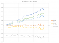
I created some new plots comparing the following solutions:
In the plots below, all the results are plotted relative to the "exact" solution. Not because I think it is the most accurate for a real plate, but rather, the most neutral, I would say. In fact, I expect that the "exact" solution would actually not be the best solution, as (I believe) it neglects shear deformation. I could be wrong about that however.
Here are the plots. In the first plot, the y axis is the predicted eigenvalues and the x axis is the "exact" solution for the same eigenvalues. In the second plot, the y axis is the percentage difference between the each solution and the "exact" solution, with the same x axis as the first graph.


Overall, I think all of the results are pretty good. Interestingly, the LISA solid model is closest to the exact solution, with the corrected FDM method being next closest but estimating slightly lower natural frequencies. The LISA shell and both Elmer models (also shell/plate elements), on the other hand, all started pretty much dead-on the exact solution but wandered higher with increasing frequency.
One curious thing is how in the second graph the profiles of all the LISA and Elmer models follow the same pattern of peaks and dips, while the FDM profile is practically a mirror image. Curious.
What's the difference between the two Elmer models? Did you guys use different mesh density? Christian's mesh was 36x121 I think, what was yours Paul? Sorry if you mentioned it, I can't recall?
For me the odd thing is that I expected that the models that include shear deformation would predict lower, rather than higher natural frequencies. That is, that neglecting shear deformation, the exact solution would act stiffer than the real panel, and hence slightly overestimate the natural frequencies. And on the other hand, the models that include shear deformation would tend to tend to give lower (and more accurate) natural frequencies than the "exact" solution.
Interestingly, for the LISA and Elmer models, the results are opposite of what I expected. Any thoughts on why?
Eric
Paul, Christian,
I created some new plots comparing the following solutions:
- "Exact" formula
- LISA Shell Elements (84x24 mesh, 2016 elements)
- LISA Solid Elements (84x24x1 mesh, 2016 elements)
- FDM (for ν=0)
- FDM (corrected by factor of (1/(1-.2^2))^0.5=1.0206, to account for ν=0.2
- Elmer (Paul)
- Elmer (Christian)
In the plots below, all the results are plotted relative to the "exact" solution. Not because I think it is the most accurate for a real plate, but rather, the most neutral, I would say. In fact, I expect that the "exact" solution would actually not be the best solution, as (I believe) it neglects shear deformation. I could be wrong about that however.
Here are the plots. In the first plot, the y axis is the predicted eigenvalues and the x axis is the "exact" solution for the same eigenvalues. In the second plot, the y axis is the percentage difference between the each solution and the "exact" solution, with the same x axis as the first graph.
Overall, I think all of the results are pretty good. Interestingly, the LISA solid model is closest to the exact solution, with the corrected FDM method being next closest but estimating slightly lower natural frequencies. The LISA shell and both Elmer models (also shell/plate elements), on the other hand, all started pretty much dead-on the exact solution but wandered higher with increasing frequency.
One curious thing is how in the second graph the profiles of all the LISA and Elmer models follow the same pattern of peaks and dips, while the FDM profile is practically a mirror image. Curious.
What's the difference between the two Elmer models? Did you guys use different mesh density? Christian's mesh was 36x121 I think, what was yours Paul? Sorry if you mentioned it, I can't recall?
For me the odd thing is that I expected that the models that include shear deformation would predict lower, rather than higher natural frequencies. That is, that neglecting shear deformation, the exact solution would act stiffer than the real panel, and hence slightly overestimate the natural frequencies. And on the other hand, the models that include shear deformation would tend to tend to give lower (and more accurate) natural frequencies than the "exact" solution.
Interestingly, for the LISA and Elmer models, the results are opposite of what I expected. Any thoughts on why?
Eric
Attachments
- Home
- Loudspeakers
- Full Range
- Application of Impulse Excitation for DML Design and Analysis