WeSaySo, thanks for the measurements.
I follow that you are comparing a conventional single driver per section system vs an array. It isn't clear why one would be so much better than the other with regard to floor bounce, yet not have greater simulated directivity. Am I misinterpreting?
I follow that you are comparing a conventional single driver per section system vs an array. It isn't clear why one would be so much better than the other with regard to floor bounce, yet not have greater simulated directivity. Am I misinterpreting?
I did the model by instantiating 75 drivers at a uniform 84 mm spacing for an extent of 3x 2.1m. That is a little bit low for anything but a basement ceiling I suppose. This puts the floor at array center, y = 0. I then set a driver offset of -1000mm. Lowering the drivers by 1m is equivalent to raising the mic 1m above the floor. No gaps at floor or ceiling or modelled. The easiest way to do this would be by muting drivers symmetrically spaced about the floor or ceiling. I modelled 2 db attenuation on floor and ceiling image drivers. My 75x TC9 line array model is attached for what it is worth. Lots of room for refinement in it. I was merely seeking an explanation for the difference between the observed vertical directivity and what simulation predicts without taking floor and ceiling reflections into account.
The question of whether or no ceiling and floor bounce suppression is worth the effort interests me. I think Toole does more than whisper. Somewhere in his book is an explicit comment that he thinks it isn't, at least not an extreme effort. The counter argument to vertical directivity is that floor bounce nulls are part of everyday life and our ears are trained to hear through them. OTOH, the dips in measured FR are hard to ignore and the engineer in me is unable to ignore them completely.
Toole's comment and the high regard in which so many conventional multiway speakers are held suggests it isn't led me in the direction of coax and cardioid with a point source of some kind at center starting more than a year ago. This approach only mitigates the boundary interference but perhaps, like you say, that is enough
Attachments
Isn't it that the sum of all the bounces results in a highly directive main beam?WeSaySo, thanks for the measurements.
I follow that you are comparing a conventional single driver per section system vs an array. It isn't clear why one would be so much better than the other with regard to floor bounce, yet not have greater simulated directivity. Am I misinterpreting?
WeSaySo, thanks for the measurements.
I follow that you are comparing a conventional single driver per section system vs an array. It isn't clear why one would be so much better than the other with regard to floor bounce, yet not have greater simulated directivity. Am I misinterpreting?
I'm guessing, but I think it has more to do with how the standards are determined/set than being a good representative in this case.
Vituixcad can present these numbers according to ANSI-CTA-2034-A, in all honesty I used 5 degree steps and a measurement
distance of 2.7 m instead of the pré-defined 10 degree and 2.0 meter. As that's the listening distance that I've used to optimize
my array results.
I wouldn't put my speaker on a Klippel and expect to see the right data come out either
 . But that doesn't mean that an array can't
be optimized to make use of the room to perform a little better and get these results. That's the whole idea. While it would be a
challenge to get that performance all the way up to the high frequencies (due to lobing), the difference I show here is just the
difference between a single 3.5" driver at 1 m height, measured at at 2.7 m listening distance, compared to an array of 25 drivers
at the same listening distance with regards to what floor and ceiling reflections do to it's frequency curve. It is clear that the array
has a slightly higher, almost similar level of reflections on the top end from about 5K up, while the array has less influence from
reflections below it.
The single driver with floor and ceiling reflections set to -6 dB:
showing the calculated ERDI of both vertical and horizontal planes.
Compared to the array of 25 drivers with the exact same settings:
Basically, what is happening is that the drivers in the array average out each other's (position dependent) reflections. More drivers means
more different driver positions with regards to averaging these results. That comes with the warning that parallel planes and ridges have
about the same distance between the plane/ridge and driver from a listening point view. So there we get no averaging out off the
reflections in those cases.
A CBT would have that extra feature, being less sensitive to the parallel planes due to the arc build (or DSP delay) making it even more room
independent than a straight array. Slightly dependent on placement of course. And maybe not as strong averaging effect due to the shading used.
Last edited:
Floor and ceiling modeled using in-room dimensions from my room with correct floor and ceiling gaps (reflection level set at -6dB)

In all honesty, using the checkmarks of the room tab in Vituixcad gives the same in-room prediction, however this can
be useful to save the resulting IR of the speaker + reflections for further research in programs like REW. It does look
remarkably close to in-room measurements (short of the wall reflections and rest of the energy in room etc). It's
quite useful as a learning tool.
Last edited:
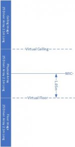
The question of where to put the listening axis when doing these floor and ceiling image arrays confuses me. I needed a visual aid as attached. With this its easy to see that with zero driver offset entered in Vituix, the listening axis is at triple array center, half the array height above virtual floor. Therefore, the graphs in the first of my two posts were the most correct. The 2nd one corresponds to near ceiling height.I did the model by instantiating 75 drivers at a uniform 84 mm spacing for an extent of 3x 2.1m. That is a little bit low for anything but a basement ceiling I suppose. This puts the floor at array center, y = 0. I then set a driver offset of -1000mm. Vituix doesn't allow a driver offset of more than 1m so I can't see what the response is beyond the edge of the main array
Attachments
nc535 said:Vituix doesn't allow a driver offset of more than 1m so I can't see what the response is beyond the edge of the main array
Vituix will let you move it 1m if you choose relocate. It will move the drivers in the table of driver layout (permanently).
After that you can move up to 1m all over again. Press relocate again if you want to go past 2m
.Here I moved up 2m24 to go above my main array height:
Top driver confirmed at -43mm (ceiling above that, floor below):
Last edited:
I'm not fully following the model but would make a couple of comments about floor and ceiling bounce. When I did a sim it was a pretty simple overall model. I was looking at an array in anechoic space. Too that I could add an array below and an array above in anechoic space but representing the floor and ceiling reflected virtual systems. I put in a typical painted drywall and carpet reflection coefficient to realistically attenuate the floor and ceiling bounce. I didn't feel that adding any other secondary reflections would be needed.
You wouldn't want to model the upper and lower arrays in addition to having some floor or ceiling bounce in your model as you would be doubling up on the floor and ceiling aspects.
Since Vituix seems to do a good room model I was expecting to see a large array create an extreme directivity index. Roughly I would expect doubling the number of elements to always give 6 dB more at the listener position but only 3 dB more in total power radiation. So if we go from 1 to 2 to 4 to 8 to 16 to 32 elements, you would have 5 instances of increasing di by 3 dB. That means 15dB d.i. relative to a single driver if we can assume that all drivers add in phase for the listener (not true for all frequencies...) Are any of the sims showing a corresponding increase in d.i.?
This is generally where the direct to reflected ratio improvement comes from.
My model corresponds to what you describe in your first paragraph. Floor and ceiling reflections are disabled as they are replaced by the image drivers. My reflection coefficients were -2 db which is a round up of the 1.5 db I've heard is appropriate for dry wall. Listening distance was 4m which is less than the line length and thus nearfield. (Is that right? I forgot the nearfield/farfield criterion but I recall it was related to line length)
The floor to ceiling array between reflective floor and ceiling approximates an infinite array. An infinite array has no directivity - its response is the same everywhere along the line. So the longer the array and the more orders of floor and ceiling reflections included in the simulated response, the better it approximates an infinite array and thus the less directivity we will see in the simulation.
I did see the increasing DI and response levels going from 25 to 50 to 75 drives but only for LFs. The effect decreased with frequency and was gone by 200 Hz. I guess the closeness of the approximation to infinite length varies with wavelength. Clearly all drivers don't add in phase at all frequencies. That may be a useful approximation at LF and definitely loses utility by the time we see combing, if not before.
Ditto on the room reflection within Vituixcad being set to off. It wouldn't make sense any other way. One can save the IR with
the mimicked reflections this way, as opposed to just having an in-room frequency curve prediction.
In all models I've shown here, EQ is being used to straighten the frequency response in room. Just as it is used in real life.
If I find the time I can make a one speaker model without EQ, 25 unshaded drivers without EQ and 25 drivers with their floor
and ceiling reflections without EQ. That should show the increase that is happening in these 25 driver arrays.
In fact, in the Vituix models one can see the EQ applied, which shows in the right middle window:

As you can see, in this example about 14 dB is shaved off at 200 Hz. In real life I shave about 10 dB off at the max output
around 200-250 Hz and use boost on the top and bottom end. Similar to what was done by Roger Russell on the IDS-25,
with the difference that these days we don't use an analog equalizer but do it with FIR processing based on in-room
measurements. I've used it playing full range with the array baffle about 50 cm from the back wall, giving a nice boost on
the low end. These days I use a couple of subs and limit (but still use some of) the bottom end.

The poster behind the listener as well as behind both of the curtains are huge damping panels. A PC controls the EQ.
**Some graphs may not show the EQ as clearly, as we've made some ABEC driver/enclosure simulations that were done
down to 200 Hz and up to 10 KHz. Vituixcad just extends and interpolates the results above and below.**
Does that make it a bit more clear what is shown here? Indeed the array effect is shown, but hidden from sight perhaps.
the mimicked reflections this way, as opposed to just having an in-room frequency curve prediction.
In all models I've shown here, EQ is being used to straighten the frequency response in room. Just as it is used in real life.
If I find the time I can make a one speaker model without EQ, 25 unshaded drivers without EQ and 25 drivers with their floor
and ceiling reflections without EQ. That should show the increase that is happening in these 25 driver arrays.
In fact, in the Vituix models one can see the EQ applied, which shows in the right middle window:
As you can see, in this example about 14 dB is shaved off at 200 Hz. In real life I shave about 10 dB off at the max output
around 200-250 Hz and use boost on the top and bottom end. Similar to what was done by Roger Russell on the IDS-25,
with the difference that these days we don't use an analog equalizer but do it with FIR processing based on in-room
measurements. I've used it playing full range with the array baffle about 50 cm from the back wall, giving a nice boost on
the low end. These days I use a couple of subs and limit (but still use some of) the bottom end.
The poster behind the listener as well as behind both of the curtains are huge damping panels. A PC controls the EQ.
**Some graphs may not show the EQ as clearly, as we've made some ABEC driver/enclosure simulations that were done
down to 200 Hz and up to 10 KHz. Vituixcad just extends and interpolates the results above and below.**
Does that make it a bit more clear what is shown here? Indeed the array effect is shown, but hidden from sight perhaps.
If I find the time I can make a one speaker model without EQ, 25 unshaded drivers without EQ and 25 drivers with their floor
and ceiling reflections without EQ. That should show the increase that is happening in these 25 driver arrays.
I did find the time to create the model for the unshaded TC9, first one driver, next up an array of 25 drivers and last but not least,
the 25 driver array with it's floor and ceiling reflection. I've kept the damping of floor and ceiling at -6 dB, as that has been used
in all my previous simulations that I've shown. I think I once checked the level that came closest to reality when comparing to real
measurements, which was a 4 dB drop but the differences between that and this picture are negligible. Lots of pictures I've shown
in this thread were old experiments I had on my harddrive, in those sims I clearly played a lot with the 6 dB reduction
.As can be seen, there is a hinge point at 5 KHz where the single driver and the array have an near equal SPL level.
At about 250 Hz we see an increase of about 13 dB. This corresponds with theory. above it we see the ~3 dB drop per
octave that is predicted in the line theory. Above 5 KHz, where combing and lobing takes it's toll it isn't any more efficient
than a single driver. However, each driver in the line only gets a fraction of the total power compared to the single driver.
Due to that reduction, it can handle higher total power which creates headroom for some EQ.
As soon as the floor and ceiling mirrors are added (with my room dimensions, ceiling being almost 3 m high after a
recent remodeling) we see an increase of 4 dB at 20 Hz, but not much more elsewhere. Up until 5 KHz hardly anything
changes, and above that we get the effects of the lobing that creates the early floor and ceiling reflections. It's clear that
the gaps between the array and floor (which makes the distance to it's mirror driver about 300mm instead of the CTC of
the array of 85.5mm) and the even larger gap between the top driver of the array and the ceiling mirror (almost 1.5 meter)
create enough discrepancy to interrupt a further increase.
I used to have a lower metal ceiling (aluminum) below the old original gypsum ceiling. I don't know what is worse, the
higher ceiling I have now or that metal ringing while taking measurements
.Yes, I guess there would be 3 zones of operation. For lowest frequencies the elements would all add in phase but the "more gain on axis" part goes away. If the elements are physically close to each other (wavelenghts are long) then the 6 dB gain from doubling elements occurs in all directions and no directivity increase happens.I did see the increasing DI and response levels going from 25 to 50 to 75 drives but only for LFs. The effect decreased with frequency and was gone by 200 Hz. I guess the closeness of the approximation to infinite length varies with wavelength. Clearly all drivers don't add in phase at all frequencies. That may be a useful approximation at LF and definitely loses utility by the time we see combing, if not before.
In the second group of frequencies there is a 6dB gain on axis but only an average of 3 dB elsewhere so increased d.i. is assumed. At frequencies still farther up the nearfield effect takes over and outermost elements of the array will not be adding in phase. I showed this in my paper as draw away curves from the center of a longer array and you could see a periodic ripple in level that persisted until the top and bottom most elements were largely in phase. From that distance out the array is no longer "long" and response starts to drop 6 dB per distance doubling where before it had been 3. There is a diagram in the paper that should make that clear.
Hi WeSaySo,I did find the time to create the model for the unshaded TC9, first one driver, next up an array of 25 drivers and last but not least,
the 25 driver array with it's floor and ceiling reflection. I've kept the damping of floor and ceiling at -6 dB, as that has been used
in all my previous simulations that I've shown. I think I once checked the level that came closest to reality when comparing to real
measurements, which was a 4 dB drop but the differences between that and this picture are negligible. Lots of pictures I've shown
in this thread were old experiments I had on my harddrive, in those sims I clearly played a lot with the 6 dB reduction
View attachment 1078609
As can be seen, there is a hinge point at 5 KHz where the single driver and the array have an near equal SPL level.
At about 250 Hz we see an increase of about 13 dB. This corresponds with theory. above it we see the ~3 dB drop per
octave that is predicted in the line theory. Above 5 KHz, where combing and lobing takes it's toll it isn't any more efficient
than a single driver. However, each driver in the line only gets a fraction of the total power compared to the single driver.
Due to that reduction, it can handle higher total power which creates headroom for some EQ.
As soon as the floor and ceiling mirrors are added (with my room dimensions, ceiling being almost 3 m high after a
recent remodeling) we see an increase of 4 dB at 20 Hz, but not much more elsewhere. Up until 5 KHz hardly anything
changes, and above that we get the effects of the lobing that creates the early floor and ceiling reflections. It's clear that
the gaps between the array and floor (which makes the distance to it's mirror driver about 300mm instead of the CTC of
the array of 85.5mm) and the even larger gap between the top driver of the array and the ceiling mirror (almost 1.5 meter)
create enough discrepancy to interrupt a further increase.
I used to have a lower metal ceiling (aluminum) below the old original gypsum ceiling. I don't know what is worse, the
higher ceiling I have now or that metal ringing while taking measurements
Your sims are starting to make more sense to me. Very constant directivity for the array from 200 on up. Spacing related aliasing at 4kHz. Not a huge benefit from adding the floor and ceiling bounce (although they are there in reality).
I'm still kind of hung up on expecting a big d.i. increase. The hinge point at 5kHz is again the frequency where the ends of the array are enough farther away to shift into random phase adding so you lose a little level in spite of the multiple elements. This is a nearfield phenom. while in the far field all elements add in phase for a straight array. The comb filter above 8k is the same poor adding from the ends of the array. This is the cause of the "sis sis sis sis" effect from raising or lowering your observation point that I notice on the Mac arrays, at least on pink noise.
Seeing the huge low/mid gains shows, to me, the big benefit of such a multielement array.
I'd say making it act largely independent from floor and ceiling was my goal and the unfiltered array almost got me there. Wanting to try if I could get a bit more got me on the simulation bandwagon with @nc535. That's when I ended up filtering the array at higher frequencies, you get rid of the comb filter nulls, however the lobing will still be present but reduced.
It's slightly less affected by floor and ceiling reflections than the unfiltered array and the top end is almost comb free. Even throughout the midrange, the effect of reduced floor and ceiling energy is noticeable and it results in even less frequency deviation if one moves up, down or left and right. Which can be seen how closely the listening window follows the main frequency curve (the dotted olive colored line slightly below the frequency curve).

It's slightly less affected by floor and ceiling reflections than the unfiltered array and the top end is almost comb free. Even throughout the midrange, the effect of reduced floor and ceiling energy is noticeable and it results in even less frequency deviation if one moves up, down or left and right. Which can be seen how closely the listening window follows the main frequency curve (the dotted olive colored line slightly below the frequency curve).
Last edited:
Probably a good time to add part 3 of the '97 paper.
You'll remember that the far field model wasn't really giving realistic results for the longer Mac array. It seemed like a nearfield model was needed.
Figure 25 defines the nearfield geometry. While in the far field you only see phase shift between elements as you move off the horizontal axis. In the nearfield you must also account for level shift and extra phase shift since the end points of the array may be swinging nearer or farther as the array is rotated.
At this point I decided that I didn't want to work in polar coordinates. The realistic case for an audiophile line array is to predict the response at a reasonable distance (2 to 3 meters) and a a variety of heights, such as seated and standing. We modified the program to add the extra elements and to allow a variation of observing height from the array center and upwards in a straight line rather than an arc. We could also set a flag where the position sweep became from near to far on the center line of the array. This would allow "draw away" curves and reveal what the near field to far field variation was.
I had spent some time comparing nearfield to far field variation and gave 2 examples of the 4kHz 23 element prediction. This brought clarity to the big difference between measurements of the 23 element array and the previous far field predictions that showed excessive directivity and nulls. I did the 4 kHz plots in 2 ways. In every case each subsequent curve was at double the distance of the previous. Levels are not normalized but show the predicted level due to distance and number of elements.For one family of curves each curve was a vertical sweep from 0 mm (array middle) to 1.5 m up. In that family (Fig. 26) the top most curve is very good at showing that level is approximately uniform up to the top of the array at about .75 m. Figure 27 plots the predicted response against a pseudo angular scale (described int the text) that is very good at showing how the nearfield response transitions to the far field. From about the 3rd curve down you can see the rough final shape. As you go farther in that direction the nulls get more severe and the narrowness of the first lobe maximizes.
The next section of the paper shows the draw away curves. These would be a single tone (1k, 3.2 k, and 10k in figures 28, 29 and 30). All had a similar characteristic where they fell roughly 3 dB per distance doubling (as expected of a line source) and when through a periodic ripple. At some distance the ripple stops and the curve starts to fall at 6dB per distance doubling. This is described in figure 31 where the ripple appears to be the outer elements going in and out of phase (inner elements are largely uniform in distance) until the outermost elements are largely in phase with all the center elements and no more ripple can occur. This was a neat realization to me and I don't believe that anything had been published on this phenomenon previously.
Attachments
I'm working on a spreadsheet version of my 23 tweeter model. It will be a nearfield model with a plot of response versus vertical rise, any frequency, any listening distance.
Maybe have something in a few days.
Does anyone out there have talents in other types of programming that would like to work up a model? I can give guidance on the acoustics part of it.
David
Maybe have something in a few days.
Does anyone out there have talents in other types of programming that would like to work up a model? I can give guidance on the acoustics part of it.
David
Have you read Harry Olson's "Acoustical Engineering" or "Music, Physics and Engineering"? Both of those address line arrays.After years of designing various types of line arrays at McIntosh, Snell and Bose, I thought I would start a conversation about what I've learned over the years, specifically in how simple modeling can lead to an understanding of line array phenomena.
While I am not a Matlab wiz I have found that Excel is good for modeling simple arrays and will give you a good understanding of what is going on. Through some simple models I intend to illustrate all of the line array phenomona and explain their root causes. Through an understanding of basic phenomona we can take steps to control polar patterns and achieve the performance that we might want.
This is not going to be a discussion about "if I put 10 Vifa units in a row, will that sound real good?". What this is is more about "what causes the lobing ('lobe-ing") and how do I control it?"or "What determines my vertical directivity?".
Hopefully some will find this interesting and those of you that are better at mathematical modeling than me may be inspired to work up some better array models than I have.
How do we calculate the performance of a line array. The basic array model
Lets say we have the simplest possible line array, 2 elements set some small distance apart. If we stack them in a vertical line and then go out from the elements and upwards so that we are 30 degrees above the elements, then how would we calculate the response of the pair of elements? Or if we want to know the polar response for some frequency, how would we calculate that?
The basic premise of array modeling is that the individual elements can be thought of as vectors that are added in space. They are assumed to be independent of each other (i.e. no mutual coupling or other interactions) but the phase of each element must be taken into account. If we take our geometry and calculate the distance difference as viewed from our 30 degree observation point, take that distance difference and convert it to a phase difference we can predict response. All we have to do is think of the 2 elements as 2 vectors with some relative phase shift between them that we (vectorially) add to get a combined array response.
If you don't remember how to add vectors it is quite simple. Start with a magnitude and phase for each element and then convert to rectangular format (using cosines and sines of the angle) and them add the "real" parts and the "imaginary" parts together. The Pythagorean Theorem will then let us convert that back to a magnitude. Once added we can convert the results to dB if desired. This is really all the spreadsheet does.
I'll confess that I am not Matlab proficient so I like to use excel to set up spreadsheets for any particular array. I've included a 2 element polar curve example. In this example column A gives the viewing angle that steps from 0 to 358 in 2 degree steps. Columns D and E define the actual geometry that defines the excess path length of each element (here only 2 elements). This is the calculation of phase difference between the 2 units. Columns H and J define real part of the radians of delay, L and M the imaginary, and P through T the magnitude of the pythagorean theorum sum. By breaking into real and imaginary parts we can sum any number of vectors as called for by the complexity of our array.
So the desired result is column T that is plotted as an Excel "radar" plot. This is an overhead view of the typical array. Up on the graph is 0 degrees and down is 180. In normal conditions the array directivity would have driver directivity added to it. In fact, if all elements aim in the same direction then total directivity is simply the sum of array related directivity plus driver directivity. So, typically, the front to back directivity is significant. Its never bothered me to see plots with no driver directivity, I just view that as the "second factor".
Note also that the polar plot is a cross sectional view of a solid of rotation. For one wavelength spacing as shown you would have a top like shape with a fat rim and narrower axle. (We can talk about why the rim is fatter later.)
The spreadsheet has 2 fields where you enter a number, one for Lambda (applied wavelength) and the second for "Dee" or distance between elements. Our first check of the array math working right is that when Lambda = Dee then our two units are one wavelength apart and see a full height peak at +-90 degrees. This would make sense in that rotating 2 elements to 90 degrees, with them one wavelength apart, should see them come back into phase. Something that should eventually make sense is that frequency doesn't really matter at all but the relationship between spacing and frequency is key. That is, the array definitions will always have a "Lambda/Dee" factor. Doubling Lambda and Dee at the same time will always return the same polar curve. This is just a way of saying that all arrays are scalable...
Also note that the height of the 4 peaks of our plot are all 2.00, this coming from the value of the in-phase sum of 2 unit vectors.
I've attached 4 sims with various ratios between wavelength and physical spacing.
This seems like enough to digest for our first look at array modeling so I'll let that soak in for a while and see if there are any questions or comments.
David Smith
Dear Just Dave,
Yes, I have read Olson and have both books on my bookshelf. Note that I refer to Olson in my paper and use one of his examples to confirm that my own math was working correctly. I also refer to his solution to continuous line arrays giving a Sin x/x general form and the implications of that.
Still not sure what you point is. Because Olson wrote on line arrays we shouldn't dig deeper?
Note that Olson primarily looks at continuous sources, while we are exploring multielement arrays. Olson gives no guidelines on array design. Olson doesn't discuss the connection between the element weighting function and the FFT. Olson, I don't recall, doesn't address nearfield to far field behaviour. Nor the nature of draw away curves and where the farfield starts as a function of frequency. Nor smoothing polar performance through array weighting. Nor modern techniques such as using DSP for multibeam arrays.
So, yes, I have read Olson but not found him to be the definitive source on the subject.
- Home
- Loudspeakers
- Multi-Way
- Line arrays. Understanding their behavior through simple modeling