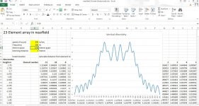
So I am pretty excited that I have the nearfield model running as I haven't done one in a spreadsheet before. For verification I've started with a copy of the 23 element Mac array as published in the 1998 paper and the new version matches exactly.
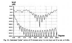
Note that the original plot shows only half of the vertical slice. I was working primarily with symmetrical arrays so a sweep from the center array up would mirror one from the center array down. The recent model shows both sides so I have encircled the top half for comparison to the old scan. Fine detail of the bumps verifies the match. The cancelation diips are a little off purely from the mismatch between plotting points losing a bit of resolution.
As a reminder of what this is, a nearfield model calculates delay and strength from every element to some not so distant observation point. In this case we have done an observation line from 4 meters away from the array and scanning from 1.75 meters below the array center to 1.75 m above. We can vary the frequency (8000 Hz shown) and the spacing of the elements (80mm). Then the scan profile shows how even the response is within the endpoints of the array (about +- 650 mm). By comparing a number of frequencies you would also have a clue as to how frequency response would be varying at some observation height. This is an anechoic model and shows response of ideal elements.
The sharp eyed will see that the new plot has both a blue and an orange plot. I "evolved" the spreadsheet initially without having near to far dB level (drop vs. distance) worked in and then added some equations to capture it. I have plotted both to show the added effect of element distance on response and was surprised with how little it matters. Orange is the true response and only shows a little bit of loss at the extremes of observation height. This may not be true for all length arrays or all observation distances (its likely to become more different if you approached the array to unnaturally close).
Not something I expected.
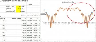
I will clean up the spreadsheet and attach it later. I really recommend that you download it and play with the variables at it is very instructional. You can play with element spacing, frequency of interest and listening distance. You will see at low frequencies that the the response gets very rounded and falls off for high and low observation levels. For mid to upper frequencies the "uniform between the endpoints of the array" response looks pretty good and then at high frequencies it becomes a comb filter mess.
After the dust settles I will add the possibility of weighting coefficients for each element which will show some of the thinking behind the shorter 16 element array we did at Mac. As you can weight some elements as "zero" you would be able to change the effective array length and model up whatever interests you.
Nobody interested in programing this into something more modern?
David
Note that the original plot shows only half of the vertical slice. I was working primarily with symmetrical arrays so a sweep from the center array up would mirror one from the center array down. The recent model shows both sides so I have encircled the top half for comparison to the old scan. Fine detail of the bumps verifies the match. The cancelation diips are a little off purely from the mismatch between plotting points losing a bit of resolution.
As a reminder of what this is, a nearfield model calculates delay and strength from every element to some not so distant observation point. In this case we have done an observation line from 4 meters away from the array and scanning from 1.75 meters below the array center to 1.75 m above. We can vary the frequency (8000 Hz shown) and the spacing of the elements (80mm). Then the scan profile shows how even the response is within the endpoints of the array (about +- 650 mm). By comparing a number of frequencies you would also have a clue as to how frequency response would be varying at some observation height. This is an anechoic model and shows response of ideal elements.
The sharp eyed will see that the new plot has both a blue and an orange plot. I "evolved" the spreadsheet initially without having near to far dB level (drop vs. distance) worked in and then added some equations to capture it. I have plotted both to show the added effect of element distance on response and was surprised with how little it matters. Orange is the true response and only shows a little bit of loss at the extremes of observation height. This may not be true for all length arrays or all observation distances (its likely to become more different if you approached the array to unnaturally close).
Not something I expected.
I will clean up the spreadsheet and attach it later. I really recommend that you download it and play with the variables at it is very instructional. You can play with element spacing, frequency of interest and listening distance. You will see at low frequencies that the the response gets very rounded and falls off for high and low observation levels. For mid to upper frequencies the "uniform between the endpoints of the array" response looks pretty good and then at high frequencies it becomes a comb filter mess.
After the dust settles I will add the possibility of weighting coefficients for each element which will show some of the thinking behind the shorter 16 element array we did at Mac. As you can weight some elements as "zero" you would be able to change the effective array length and model up whatever interests you.
Nobody interested in programing this into something more modern?
David
Attachments
Here is the nearfield spreadsheet for the 23 tweeter array. Hopefully someone can open it up and confirm that it works.
As before the yellow fields in the upper left corner are numbers you can change (actually speed of sound is a dummy). Frequency is self explanatory. Element spacing is the center to center between your drivers. 0.08 meters was the spacing of the McIntosh 1" dome tweeters. Note that if you change element spacing your are also changing the length of the array as the array element quantity is constant. Listening distance is the perpendicular distance from the line array to the listener location.
The plot is kind of sideways but represents the pressure level observed if you traversed a mic from 1.75 meter below the center of the array to 1.75 meter above. It is like a vertical polar curve except it is in rectangular coordinates rather than having the mic swing in an arc. This seems more useful for an array in the living room where you may sit or stand.
As I said before, open the spreadsheet and play with the numbers. I am surprised at how much listening distance can impact response. For example the current settings of 8000 Hz, .08m, 4 meters distance looks reasonable with a flat top across the length of the array (from about -.75 to +.75). If you cut the listening distance down to 2 meters then the response turns to **** with constant comb filtering and no particular plateau.
Enjoy.
Attachments
Hopefully someone can open it up and confirm that it works.
I can confirm the spreadsheet works as expected in Excel on a Windows PC.
")
I can change the values in yellow, I did not try to alter the speed of sound
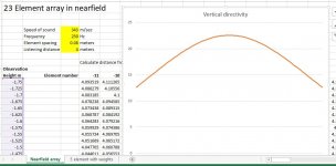
.Here are some examples of the 23 element array over a range of frequencies. Although we are looking at a particular spacing, observation distance and element qty., this is very typical of any long multi-element straight array.

At low frequencies the array vertical performance is smooth and has some directivity in line with the array length.

Same thing for 500 Hz but a little narrower, Still a smooth Gaussian looking vertical directivity.
Note that the axial response peaks at a level of around 22. The program does not normalize so this is a value close to the peak of 23 elements. i.e. all elements are largely in-phase.

Lots of ripple at 1000 Hz and overall narrower response. Peak level around 19 so some cancellation is going on.
At low frequencies the array vertical performance is smooth and has some directivity in line with the array length.
Same thing for 500 Hz but a little narrower, Still a smooth Gaussian looking vertical directivity.
Note that the axial response peaks at a level of around 22. The program does not normalize so this is a value close to the peak of 23 elements. i.e. all elements are largely in-phase.
Lots of ripple at 1000 Hz and overall narrower response. Peak level around 19 so some cancellation is going on.
Attachments
(Carrying on)

At 2000 Hz it really starts to square up. This is the "response is uniform within the end points of the array" region. Note that the max level is now under 12.

5000 Hz is getting a little ugly but is still essentially a square top. Note that the top level is now down to about 7. If we averaged the center sections and plotted them vs. frequency then we would have the array related frequency response. It has now drooped from about 23 down to 7, meaning that the array would tilt from max gain at low frequencies to quite a bit less here.

Yuch! (I used a different expletive earlier but it turned it to ****)
At 10kHz we have lost our forward beam and just have a mess of ripple. What has most likely happened here is that strong side lobes formed at 90 degrees (as they always do when the element spacing approaches 1 wavelength) and the lobes fold inward at higher frequencies. This makes the forward response looke like 3 wide lobes in a row and no particular directivity is left.
Can we do better? Are the lobes inevitable? (aliasing?) Would weighting help? Frequency dependent weighting?
(Send answers on a postcard along with $5.00 to...)
David
At 2000 Hz it really starts to square up. This is the "response is uniform within the end points of the array" region. Note that the max level is now under 12.
5000 Hz is getting a little ugly but is still essentially a square top. Note that the top level is now down to about 7. If we averaged the center sections and plotted them vs. frequency then we would have the array related frequency response. It has now drooped from about 23 down to 7, meaning that the array would tilt from max gain at low frequencies to quite a bit less here.
Yuch! (I used a different expletive earlier but it turned it to ****)
At 10kHz we have lost our forward beam and just have a mess of ripple. What has most likely happened here is that strong side lobes formed at 90 degrees (as they always do when the element spacing approaches 1 wavelength) and the lobes fold inward at higher frequencies. This makes the forward response looke like 3 wide lobes in a row and no particular directivity is left.
Can we do better? Are the lobes inevitable? (aliasing?) Would weighting help? Frequency dependent weighting?
(Send answers on a postcard along with $5.00 to...)
David
I've got a lot of code that could probably improve on the spreadsheet results, by adding a piston source model, graphical tools to locate drivers, and a crossover overlay for 2 or 3-way line arrays. However, that code was written at least 10 years ago using VB.NET. That code still compiles in Visual Studio, but I promised myself I wouldn't continue down that path. It is not just that it isn't in a more "popular" programming language--it is because that approach isn't sufficient to illustrate what I really want to see in a line array model.
For me, the primary attraction of the line array is what has been mentioned several times in this thread: that the response falls off at a 3dB rate for doubling the distance, rather than 6dB. That response results in a very different spatial image that I find satisfying. I like the way the line array fills up the listening space and provides a convincing stereo image from many listening positions. However, I don't see any good way to model these spatial images using 2D renderings, so I started looking at the tutorials for Unity to get some ideas for rendering in 3D.
Obviously, the numbers of vectors involved will be massive for a 3D spatial model, so I bought a good 3D card to see whether the ray tracing could accelerate the number-crunching. AMD's RX6000 series supposedly supports audio ray tracing using Ambisonics (see this link), so I bought one of those cards to encourage myself to explore audio 3D modeling. I don't play computer games--that's the primary reason I got that card, along with VR glasses. Realistically, I'll never get to it before I pass away at the rate I'm going, but at least I don't have any excuses for not taking a stab at a 3D audio model.
For me, the primary attraction of the line array is what has been mentioned several times in this thread: that the response falls off at a 3dB rate for doubling the distance, rather than 6dB. That response results in a very different spatial image that I find satisfying. I like the way the line array fills up the listening space and provides a convincing stereo image from many listening positions. However, I don't see any good way to model these spatial images using 2D renderings, so I started looking at the tutorials for Unity to get some ideas for rendering in 3D.
Obviously, the numbers of vectors involved will be massive for a 3D spatial model, so I bought a good 3D card to see whether the ray tracing could accelerate the number-crunching. AMD's RX6000 series supposedly supports audio ray tracing using Ambisonics (see this link), so I bought one of those cards to encourage myself to explore audio 3D modeling. I don't play computer games--that's the primary reason I got that card, along with VR glasses. Realistically, I'll never get to it before I pass away at the rate I'm going, but at least I don't have any excuses for not taking a stab at a 3D audio model
.Ambitious project there, Neil! I do hope you get going with this at some point .
@speaker dave, I do hope your next step in this thread will be the expanding array. Any luck with Vituixcad yet?
And how many postcards did you get. It's quiet in here...
.@speaker dave, I do hope your next step in this thread will be the expanding array. Any luck with Vituixcad yet?
And how many postcards did you get
. It's quiet in here...Hi WeSaySo,
It is quiet here but I am about to add a layer to the near field model. There is still a step or two before getting to the expanding array. (Patience)
I have done a little with Vituixcad. I have used enough network simulators that much of it feels familiar. I want to do some hypothetical expanding arrays but need driver models. Are there any good sources for off the shelf driver models?
Neil, I would love to see more of your work. (Hoping for more contributions from those observing the thread.)
The last spread sheet took the 23 element array and created a nearfield model. As this appears to be accurate relative to measurements of the McIntosh array, I have added a means of applying weighting coefficients for each element. This is in the form of strength multipliers. This is a half step to frequency dependent weighting, a fancy term for applying filters to each element. If an array performs well at one frequency with one weighting profile and needs another weighting profile to give what you want at another frequency, then you have just defined 2 points of a filter response for each element.
Let me give some examples to try to make some sense of that.

First, see that the above spreadsheet (based on the last one from a few weeks ago) now has a horizontal row for weighting coefficients. These are above the first rows for the elements represented just below by -11 to +11. The weighting coefficients can be anything in a wide range but I tend to use 1 as the full strength coefficient and a few other select values such as 0.7 for about 3dB down, 0.5 for -6, 0.3 for -10dB and 0.1 for -20. You could go lower but at -20dB the contribution of an element is minimal (as in, leave a gap and save some money). You can also simulate arrays of any length from 1 to 23 elements. That is, if the first 5 and last 5 elements are 0.0 then you are really modeling a 13 element array. Note that you can model even number arrays but you will have a slight shift in the array centering.
It shouldn't be a big surprise that changing the profile by gradually rolling off the first and last elements tends to give a smoother and better behaved polar response. This was the big takeaway from the 16 element array that I did at Mac. I called the weighting of the Mac array a raised cosine profile, but it was really just a smoothly rolled off profile to the top and bottom elements. More on that later.

Here are 2 log plotted vertical response profiles. Remember that these are a scan of from 1.75 meters above the array center line to 1.75 m below. I suppose that rotating it 90 degrees clockwise would make it a little easier to picture (excel...) We can see a smooth polar with approximately even response level from 0.5 meter above to 0.5 meter below its center line.
Now these 2 plots, quite similar except for level, are plots of 2 different profiles at 2 different frequencies. The orange curve is 1000 Hz while the blue curve is 2000 Hz. How do we achieve the same vertical polar at 2 different frequencies? Remember that arrays are always scalable. If you want a given array to look the same an octave lower then you simply scale it to be twice as big (you expand it...).
The weighting profiles were as follows:
0.1 0.1 0.3 0.3 0.5 0.5 0.7 0.7 1 1 1 1 1 1 1 0.7 0.7 0.5 0.5 0.3 0.3 0.1 0.1 was used for 1000Hz (orange curve).
the second version for 2000 Hz (blue) was:
0 0 0 0 0 0 0.1 0.3 0.5 0.7 1 1 1 0. 7 0.5 0.3 0.1 0 0 0 0 0 0
Note that the 2000 Hz profile has starting and ending zeros such that its final effective length is, due to only 11 active elements, roughly cutting its length in half. This is how we can have the same vertical directivity as 2 different frequencies an octave apart. The shorter array length leads to lower response level (fewer elements playing at full strength).
This should suggest how we could achieve constant directivity over a wide range. Simply expand the weighting profile in proportion to wavelength as you go down in frequency, shrink it as you go up. In frequency terms this suggests that giving each element a 6dB per octave rolloff with corner frequencies in proportion to its distance from the array center is all you need to do!
The directivity that the above illustrates isn't magical. If you wanted a more directional array then you would just shoot for a longer weighting profile for a given frequency. A shorter profile (fewer active elements) would give broader polar response. The key is making it proportional to radiated wavelength for as wide a frequency range as possible.
Also remember that we are creating a sampled array rather than a continuous one. That means that at higher frequencies aliasing (lobes) will always raise their ugly head. It is, of course, possible to crossover at higher frequencies to a shorter but denser array (say, 7 or 9 dome tweeters close together crossing over to a similar number of more broadly spaced mids).
Let me let this all sink in for a while before we move on.
Let me give some examples to try to make some sense of that.
First, see that the above spreadsheet (based on the last one from a few weeks ago) now has a horizontal row for weighting coefficients. These are above the first rows for the elements represented just below by -11 to +11. The weighting coefficients can be anything in a wide range but I tend to use 1 as the full strength coefficient and a few other select values such as 0.7 for about 3dB down, 0.5 for -6, 0.3 for -10dB and 0.1 for -20. You could go lower but at -20dB the contribution of an element is minimal (as in, leave a gap and save some money). You can also simulate arrays of any length from 1 to 23 elements. That is, if the first 5 and last 5 elements are 0.0 then you are really modeling a 13 element array. Note that you can model even number arrays but you will have a slight shift in the array centering.
It shouldn't be a big surprise that changing the profile by gradually rolling off the first and last elements tends to give a smoother and better behaved polar response. This was the big takeaway from the 16 element array that I did at Mac. I called the weighting of the Mac array a raised cosine profile, but it was really just a smoothly rolled off profile to the top and bottom elements. More on that later.
Here are 2 log plotted vertical response profiles. Remember that these are a scan of from 1.75 meters above the array center line to 1.75 m below. I suppose that rotating it 90 degrees clockwise would make it a little easier to picture (excel...) We can see a smooth polar with approximately even response level from 0.5 meter above to 0.5 meter below its center line.
Now these 2 plots, quite similar except for level, are plots of 2 different profiles at 2 different frequencies. The orange curve is 1000 Hz while the blue curve is 2000 Hz. How do we achieve the same vertical polar at 2 different frequencies? Remember that arrays are always scalable. If you want a given array to look the same an octave lower then you simply scale it to be twice as big (you expand it...).
The weighting profiles were as follows:
0.1 0.1 0.3 0.3 0.5 0.5 0.7 0.7 1 1 1 1 1 1 1 0.7 0.7 0.5 0.5 0.3 0.3 0.1 0.1 was used for 1000Hz (orange curve).
the second version for 2000 Hz (blue) was:
0 0 0 0 0 0 0.1 0.3 0.5 0.7 1 1 1 0. 7 0.5 0.3 0.1 0 0 0 0 0 0
Note that the 2000 Hz profile has starting and ending zeros such that its final effective length is, due to only 11 active elements, roughly cutting its length in half. This is how we can have the same vertical directivity as 2 different frequencies an octave apart. The shorter array length leads to lower response level (fewer elements playing at full strength).
This should suggest how we could achieve constant directivity over a wide range. Simply expand the weighting profile in proportion to wavelength as you go down in frequency, shrink it as you go up. In frequency terms this suggests that giving each element a 6dB per octave rolloff with corner frequencies in proportion to its distance from the array center is all you need to do!
The directivity that the above illustrates isn't magical. If you wanted a more directional array then you would just shoot for a longer weighting profile for a given frequency. A shorter profile (fewer active elements) would give broader polar response. The key is making it proportional to radiated wavelength for as wide a frequency range as possible.
Also remember that we are creating a sampled array rather than a continuous one. That means that at higher frequencies aliasing (lobes) will always raise their ugly head. It is, of course, possible to crossover at higher frequencies to a shorter but denser array (say, 7 or 9 dome tweeters close together crossing over to a similar number of more broadly spaced mids).
Let me let this all sink in for a while before we move on.
Ambitious project there, Neil! I do hope you get going with this at some point
@speaker dave, I do hope your next step in this thread will be the expanding array. Any luck with Vituixcad yet?
And how many postcards did you get
Note that Dave's "eXpanding Array", Horbach-Keele's array and Butterfield's Fractal Array are nearly the same thing. Arguably, the latter is the most advanced as it works in two dimensions not one.
https://www.google.com/search?q=snell+expanding+array
https://www.google.com/search?q=horbach+keele
https://www.google.com/search?q=site:diyaudio.com+fractal+array
Thanks for starting this thread…I am still catching up on all the posts. Back when I started studying line arrays, your paper provided guidance and inspiration. I created my own FORTRAN software to recreate all the plots in your paper. More recently, I realized that I could use existing polar plotting routines(like those provided by ARTA) to see how response trends with frequency and angle(or height) at the same time. For example, here is a waterfall and polar map comparison of a finite length line source, either one continuous ribbon, or made from 23 spaced tweeters as in your paper. You can easily see where the aliasing from the tweeter spacing corrupts the response of the array....remember that we are creating a sampled array rather than a continuous one. That means that at higher frequencies aliasing (lobes) will always raise their ugly head. It is, of course, possible to crossover at higher frequencies to a shorter but denser array (say, 7 or 9 dome tweeters close together crossing over to a similar number of more broadly spaced mids).


If cuts are made at 1kHz, 2Khz, 5kHz, & 10Khz you can see they line up well with your plots from Post#148-149.

As you mentioned, the frequency at which aliasing begins changes with tweeter spacing. It also changes with listening distance.


Moving on to your current topic of weighting, here are some comparisons of the Sin(x)/(x) weighting from your paper, the stepped Cosine weighting for 23 tweeters from Post#154, and a Hanning window weighting. The simple stepped weighting provides an excellent approximation of the Hanning window and provides near constant directivity from 1kHz to 10kHz where aliasing begins.

This approach is popular with segmented ESLs to provide nice smooth uniform directivity. With ESL segments being capacitive loads, a simple R-C transmission line made from a resistive ladder network provides the required progressive increments of 6dB roll-off for each segment. For ribbons or dynamic drivers with a resistive load, an inductive ladder network should work if the load impedance can be properly managed. More details in AES paper here:This should suggest how we could achieve constant directivity over a wide range. Simply expand the weighting profile in proportion to wavelength as you go down in frequency, shrink it as you go up. In frequency terms this suggests that giving each element a 6dB per octave rolloff with corner frequencies in proportion to its distance from the array center is all you need to do!
Wide-Range Electrostatic Loudspeaker with a Zero-Free Polar Response
Author: White, D. R.
Affiliation: Industrial Research Ltd, Lower Hutt, New Zealand
JAES Volume 57 Issue 10 pp. 822-831; October 2009
Publication Date: October 29, 2009
https://www.aes.org/e-lib/browse.cfm?elib=14844
Last edited:
Oh, that's great stuff bolserst. Great to see it in 3D vs. frequency and elevation. Can you tell us a bit more about your plotting approach?
I'm glad your results corroborated mine. That is a great fear of those that publish, that a major error will be found in a paper (one of the few formulas in my paper is wrong but no one has ever commented on it). Amused that you started out in Fortran. Another dinosaur out there...
I had not seen the paper on tapered drive electrostatic loudspeakers. When I was at KEF, Peter Walker of Quad would talk to us about the ESL 63 occaisionally. The marketing material describes it as delay rings to mimic a spherical sector. In reality Peter said they had to do a lot of experimental adjustments to keep the polars clean. I think the truncation of the sphere gave polar narrowing just like the midrange narrowing of a CD horn without its outer flange angle adjustment.
I have seen array weighting profiles as an academic subject but, unfortunately, not as something that has been much exploited commercially (CBT aside). As I mentioned earlier, I have brought the subject up with a few line array companies but they had no interest or understanding. The pro line array crowd is more knowledgeable and the JBL software, for example, guides you towards better responding array weighting.
Thanks again for a valuable contribution.
Sure. When I started using ARTA for measuring loudspeakers, I was really struck by the power of the 3D polar plots in visualizing what exactly was going on. It dawned on me that I could feed in simulated responses instead of just what I measured. So, created a wrapper script that would increment thru measurement angle (horizontal or vertical) or vertical height. An IFFT is performed on each of these frequency responses and a set of appropriately named ARTA formatted binary impulse files(*.pir) are created. These are then read into ARTA's polar plotting utility as a set and off you go making pretty pictures. I also included the ability to normalize the response to one particular angle(or height) or the average of, say, a 30deg window which will better match what you would get if you applied EQ to flatten the response in the listening window. I've been working at getting this all transferred over to VBA to run within Excel. It won't be quite as fast, but will be more portable. I can certainly share once complete, if anybody is interested. You would need Excel Version 2007 or newer.Oh, that's great stuff bolserst. Great to see it in 3D vs. frequency and elevation. Can you tell us a bit more about your plotting approach?
Ha! I actually still deal with FORTRAN in some parts of my day job.I'm glad your results corroborated mine. That is a great fear of those that publish, that a major error will be found in a paper (one of the few formulas in my paper is wrong but no one has ever commented on it). Amused that you started out in Fortran. Another dinosaur out there...
Concerning formula error...the copy I got from the library back in the day had a correction scribbled in the margins for summation formula on the 3rd page.
Basically, the sin(alpha) term should have been in the numerator of both cos() and sin() summation terms. I wonder if it was corrected in the online version of the paper?
Pretty amazing what Walker was able to accomplish without the help of computers and simulation capability we take for granted today. If interested, diyAudio member Hans Polak has developed an LTspice model of the complete electrical response of the ESL63. Using that electrical response, I simulated the acoustic response of the rings and created some polar plots comparing the ESL63 design(virtual point source) vs Tim Mellow's more recent Virtual Oscillating Sphere approach.I had not seen the paper on tapered drive electrostatic loudspeakers. When I was at KEF, Peter Walker of Quad would talk to us about the ESL 63 occaisionally. The marketing material describes it as delay rings to mimic a spherical sector. In reality Peter said they had to do a lot of experimental adjustments to keep the polars clean. I think the truncation of the sphere gave polar narrowing just like the midrange narrowing of a CD horn without its outer flange angle adjustment.
https://www.diyaudio.com/community/...ater-delay-line-inductors.338927/post-6239962
JAES Article on Oscillating Sphere implementation:
https://www.frontro.co.uk/s/How-do-...tic-loudspeaker-with-constant-directivity.pdf
FrontRo Loudspeaker website:
Electrostatic — FrontRo
I forgot I had written another version of the code to generate polar response animations that may be of interest. It was setup to include an overlay of point source response, so you could get a feel for how much of the polar pattern was coming from the array length/weighting and how much was coming from the size of the individual sources. Here are a few examples using configurations from your paper. The *.zip file contains *.mp4 versions if the animated gifs don't work properly, or you happen to want to pause at a particular frequency.
23 Tweeter line source with uniform weighting: Left plot @ 1000m (ie Far field), Right plot @ 4m

23 Tweeter line source with the sin(x)/x weighting: Left plot @ 1000m (ie Far field), Right plot @ 4m

5 Tweeter line source with approximate Bessel weighting (0.5, 1.0, 1.0, -1.0, 0.5): Left plot @ 1000m (ie Far field), Right plot @ 4m

23 Tweeter line source with uniform weighting: Left plot @ 1000m (ie Far field), Right plot @ 4m
23 Tweeter line source with the sin(x)/x weighting: Left plot @ 1000m (ie Far field), Right plot @ 4m
5 Tweeter line source with approximate Bessel weighting (0.5, 1.0, 1.0, -1.0, 0.5): Left plot @ 1000m (ie Far field), Right plot @ 4m
Attachments
Yes, that was the error. It was never corrected because I didn't find it until years later.
Love the animations.
I assume VBA means Visual Basic? I was looking into doing "for" loops in excel and the answer was always Visual Basic. Not sure I want to learn more languages but I would certainly like to see the results if you convert over to excel and VBA.
There is a very untapped landscape here of making better performing line arrays. The potential is high power handling from more elements and very ideal polars at a wide range of specified directivities. I hope others catch onto the potential.
- Home
- Loudspeakers
- Multi-Way
- Line arrays. Understanding their behavior through simple modeling